Augustine Atlas

Did You Know?

Surprising facts and the stories behind them.

Scroll to read. Swipe sideways for the next story.

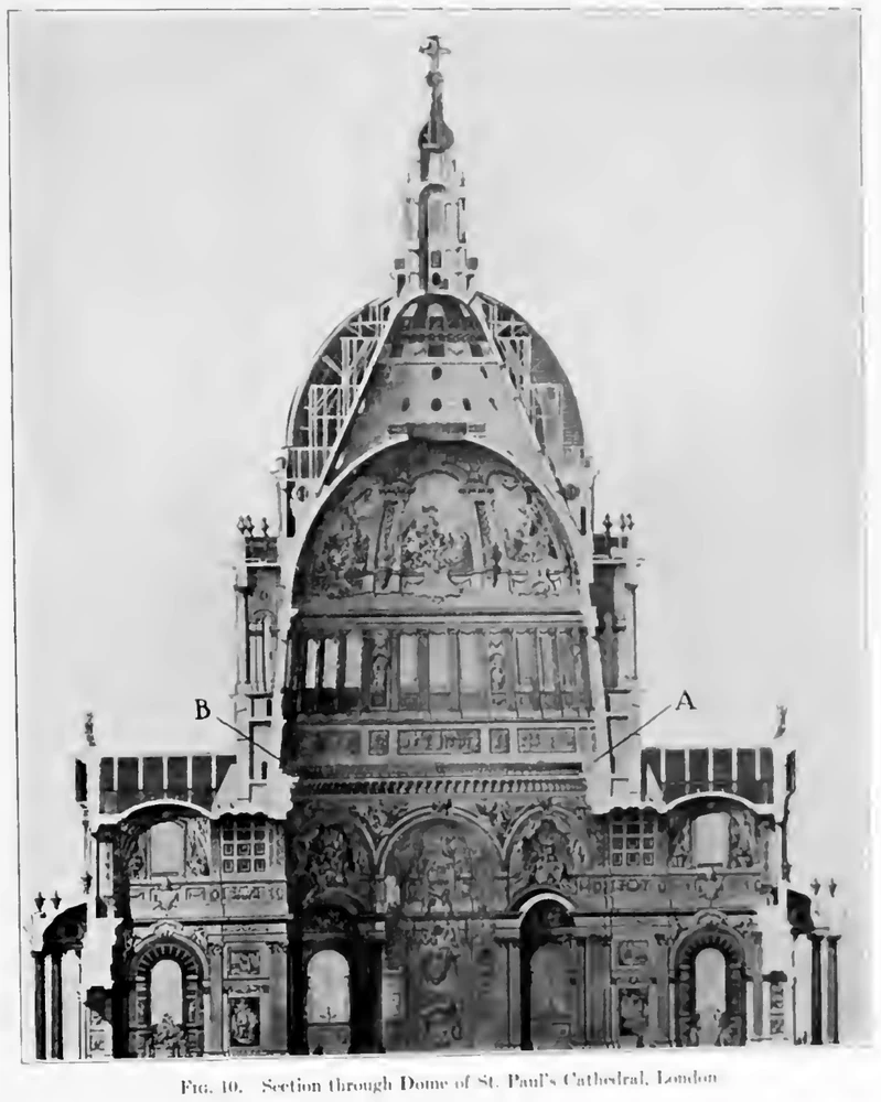
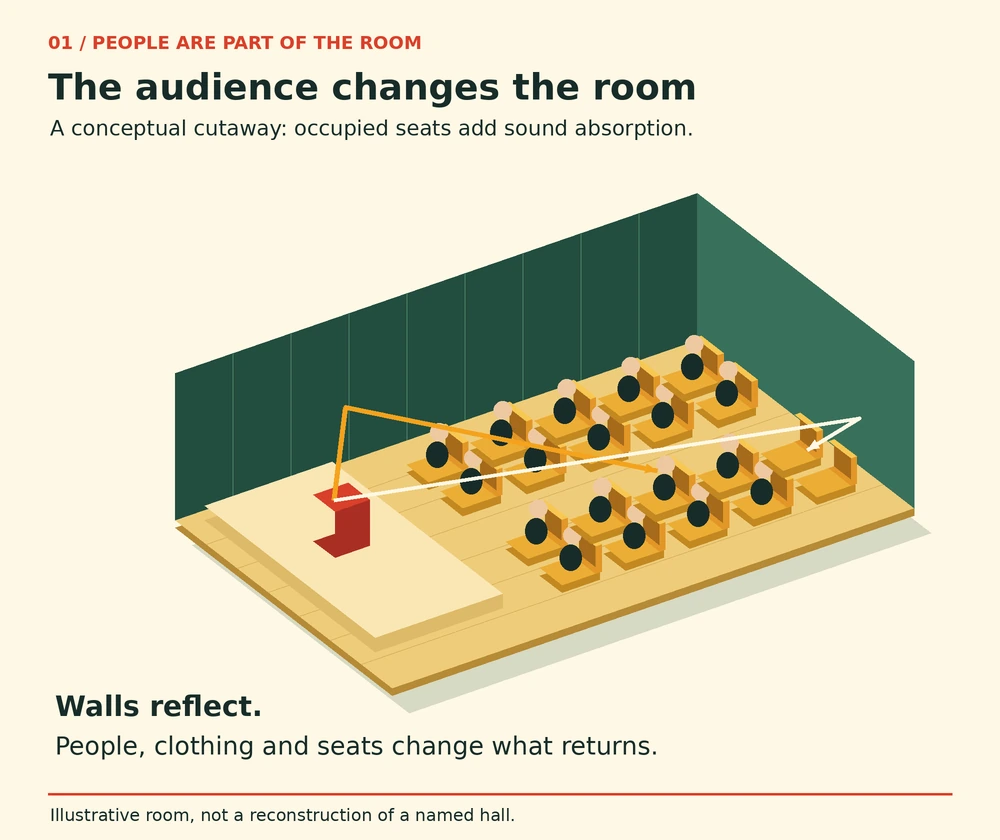
An isometric cutaway of an illustrative hall shows occupied seats, reflecting walls and two example sound paths.
Original architectural schematic. The occupied seating represents an additional acoustic part of the room. Paths are illustrative, not measured. · Augustine Atlas

Acoustics of Places · 6 min read

An audience changes a room before it makes a sound

AI narration · Maeve

An empty hall can seem to answer every small sound. A shoe scrapes, a chair moves, and a faint trail remains after the original movement has stopped. Later, people arrive and the same space can sound noticeably different. People introduce new noises, and they also change the room while sitting perfectly still. An audience changes the surfaces that sound encounters. Clothing, bodies and occupied seating become part of the room’s acoustic behavior. The listeners are therefore doing two jobs at once: hearing the performance and helping to determine the sound that reaches everyone else.

The lingering trail is reverberation. Sound leaving a source reaches a listener directly, but it also strikes walls, ceiling, floor, furniture and people. Some of its energy returns in reflections, then reflects again. Many arrivals overlap, producing a fading continuation after the source stops. A single clearly separated repeat is an echo. A dense tail of overlapping returns is a different experience. A room can have both. Reducing the energy that survives successive encounters with surfaces can shorten the tail, without changing the distance between the stage and the back row or the height of the ceiling.

Wallace Clement Sabine investigated this relationship while working on troublesome rooms at Harvard. His papers describe experiments in which seat cushions were brought into a room in increasing quantities and the duration of the remaining sound was timed. The reported Fogg lecture-room series reduced its original duration of audibility from 5.61 seconds to 0.75 second. Those historical observations reflect his particular source and listening procedure. Their significance lies in the controlled change: the room’s size stayed put while material placed inside it altered the persistence of sound.

Sabine also tested audiences directly. In the summer of 1897 he measured the residual sound in the Fogg Art Museum before and immediately after an audience left a lecture. His account records a complication rather than concealing it: rain on the roof interfered with listening. In 1899 he repeated the investigation on a more elaborate scale in the Jefferson Physical Laboratory. Three chronographs and three observers provided independent determinations. A crowded audience was measured, part of that audience departed, and the measurements were repeated. Another lecture supplied a further audience. People entering and leaving became a controlled experimental change.

Even that comparison needed care. A person does not arrive in a room containing nothing else. The occupied place already has a seat and some floor beneath it. Sabine subsequently removed the settees, measured their contribution and considered the floor area hidden by a seated audience. This is a subtle but important accounting problem: adding people also changes which existing surfaces are exposed to sound. It would be misleading to treat every listener as an entirely separate packet of absorption added to an otherwise unchanged set of visible materials. The occupied arrangement is what the room actually presents to the sound field.

His results depended on the particular audience and conditions. The papers discuss the importance of clothing and the difference between people closely seated together and people more widely separated. They also connect absorption with pitch. The useful lesson is that attendance matters and needs to be specified when describing a hall. Such comparisons depend on the source, frequency, seating, clothing and measurement conditions. A historical experiment can establish a relationship while leaving plenty of work for a modern designer who must predict a particular occupied room.

Acousticians often express absorption as an equivalent area. Imagine a surface of ten square metres that absorbs one quarter of the incident sound energy at a chosen frequency under the specified conditions. Its contribution would be 2.5 square metres of equivalent absorption area. This is an accounting example, not a claim about a particular curtain or audience. Summing contributions provides a way to compare rooms with different mixtures of surfaces. It also explains why the word area can appear in an acoustic calculation even when the question concerns people, seats and furnishings rather than a simple patch of wall.
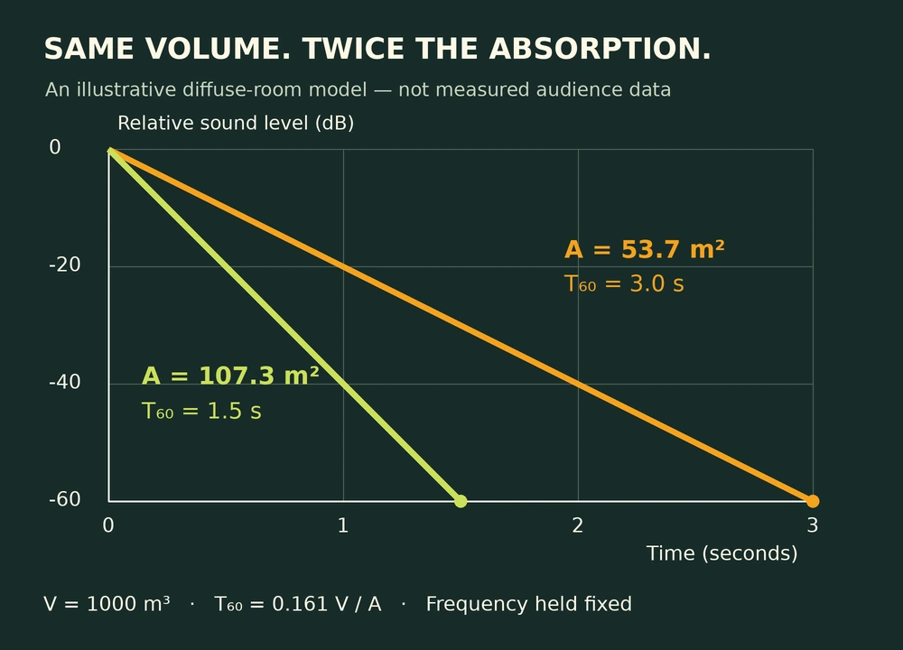
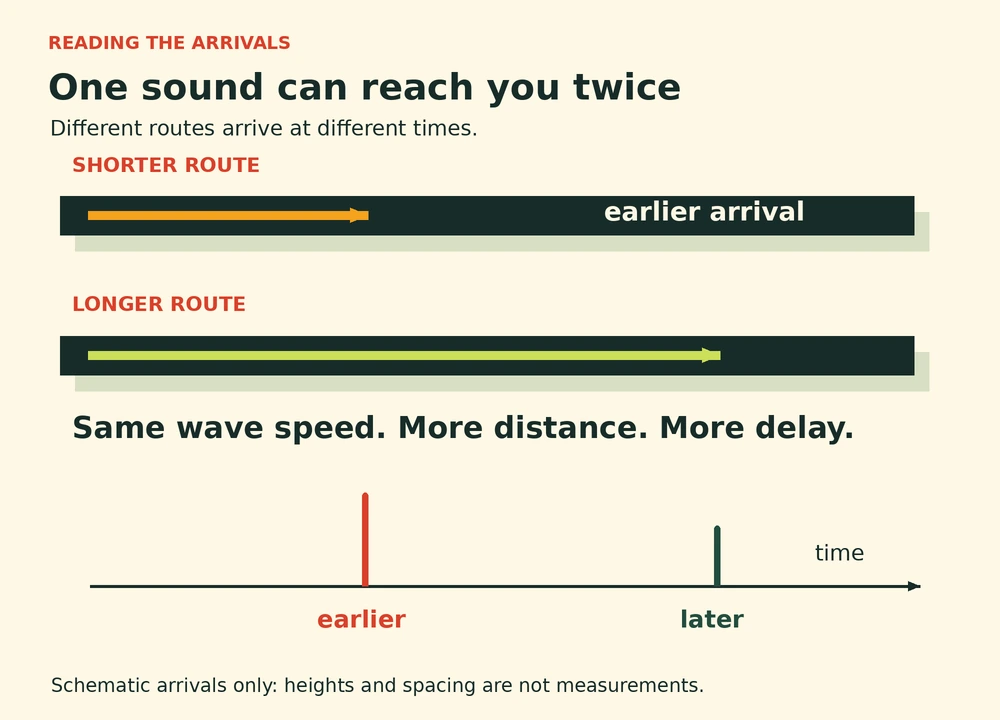
A labeled model plot shows a 60 decibel decay taking three seconds with 53.7 square metres of absorption and one and a half seconds with 107.3 square metres.
Original model plot: room volume 1000 m³, T₆₀ = 0.161 V/A, equal initial levels and a fixed frequency. This demonstrates the diffuse-room approximation, not measured audience data. · Augustine Atlas

The classic Sabine relationship connects reverberation time to room volume divided by total absorption. In an ideal diffuse-room approximation, keeping the volume fixed while doubling total absorption halves the predicted reverberation time. The accompanying plot demonstrates that relationship with invented, explicitly labeled model inputs. Both curves begin at the same normalized sound level. The steeper one reaches the same reduction sooner. Predicting an actual audience requires knowing how attendance changes the room’s total absorption. Attendance is only one contribution to absorption, and real rooms do not always satisfy the model’s assumptions.

Frequency is another reason to resist a single description such as lively or dead. Materials do not necessarily absorb a low note and a high note equally. A room can therefore have different decay times in different frequency bands. Early investigators already recognized that a change in audience could alter the balance of reverberation across musical tones. The same room might sustain some components while allowing others to fade more quickly. Describing only one overall number can hide that difference. The acoustic character heard in the seats is a combination of those frequency-dependent responses and the timing of the arrivals.

Whether a shorter tail is desirable depends on the event. In a lecture, lingering fragments can overlap later syllables and make words harder to distinguish. Sustained musical sound may benefit from some blending, although too much persistence can also obscure detail. Floyd Rowe Watson’s experimental report on the University of Illinois Auditorium explicitly discussed this compromise between speech and music. The room does not have a single best behavior independent of its use. A quiet lecture, an unamplified ensemble and a heavily amplified event ask different things of the same enclosed space and its occupied seating.

This also explains why an empty-room inspection cannot answer every question about an event. A careful description should record whether seats were occupied, what furnishing was present and which sounds were examined. Comparing an empty rehearsal with a full performance changes more than the number of listeners. It changes the acoustic system. At the same time, a crowd can introduce conversation, coughing and movement. Those additional sources are separate from the crowd’s effect on absorption. A busier room may contain more unwanted noise even while its reverberant tail becomes shorter. The two observations are compatible.

The audience is easy to overlook because it appears temporary. Stone, plaster and timber seem to belong to the building, while listeners appear to be guests passing through. Acoustically, the distinction is less tidy. During a performance, the room includes the people seated inside it and the surfaces they expose or cover. Sabine’s experiments made that changing membership measurable. A hall’s sound changes as the gathering takes shape. Each gathering completes a different version of the room, and every quiet listener contributes to the space everyone hears.
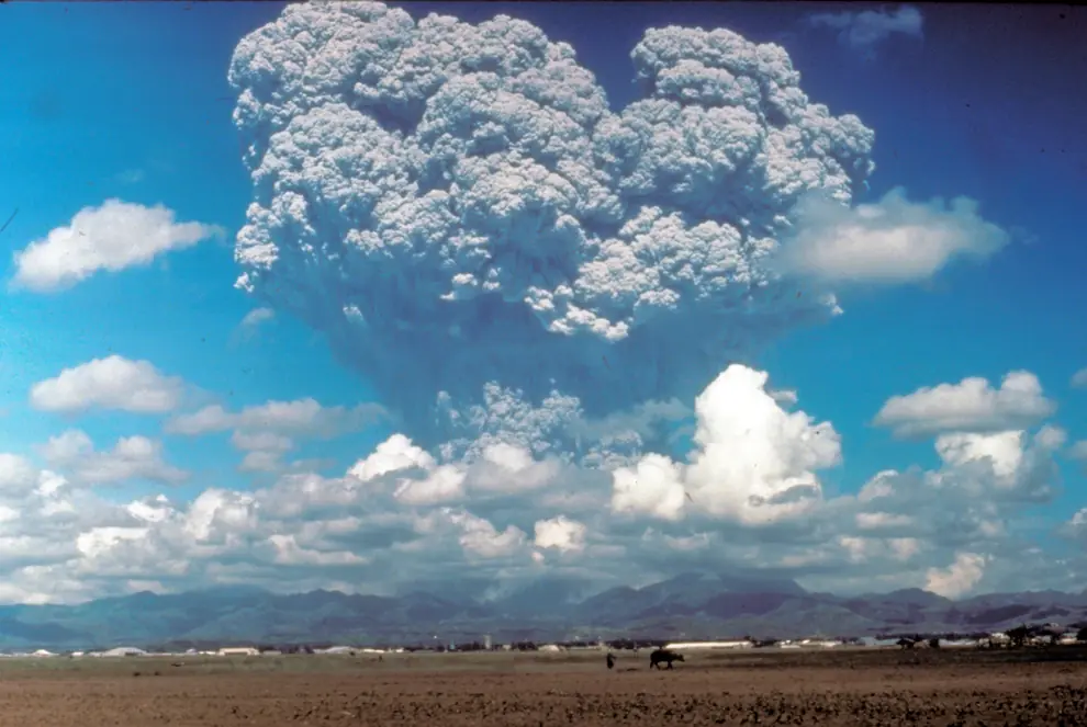

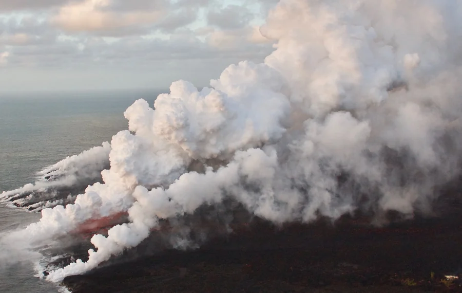
An immense gray volcanic column billows above Mount Pinatubo, rising behind low clouds and a strip of flat ground.
Dave Harlow photographed this eruption column from the east side of Clark Air Base on June 12, 1991, three days before the climactic eruption. Resized for display. · Dave Harlow · U.S. Geological Survey · U.S. public domain · 17 U.S.C. § 105

Atmospheric Aerosols · 6 min read

Pinatubo’s aerosol layer was still measurable two years later

On June 12, 1991, Dave Harlow took a photograph from the east side of Clark Air Base in the Philippines. A column from Mount Pinatubo towers behind the layer of clouds over the airfield. The climactic phase of the eruption came on June 15. By the time the most powerful columns had collapsed, clouds of material had already entered the stratosphere. Two years later, instruments were still measuring the extra particles. They could trace the disturbance far from the volcano, in atmospheric layers where most ordinary weather never reaches.

For people on Luzon, the hazards unfolded close to the ground. Ash covered land and buildings. A typhoon was passing nearby during the climactic eruption, and rainfall swept loose volcanic debris downslope in flows called lahars. Once river valleys filled with volcanic material, more rains could send damaging flows through them. The atmospheric record followed a different part of that same event. The height of the eruption column had sent some of its contents above the tropopause, the boundary between the turbulent lower atmosphere and the more stably layered stratosphere.

Sulfur dioxide helped the eruption leave such a long record. It went aloft as a gas along with ash and other volcanic materials. In the stratosphere, chemical reactions turned sulfur dioxide into sulfuric acid. The acid and water formed solution droplets. They could grow as more material condensed onto them and as particles collided and joined. Aircraft and balloon measurements contributed to the picture of what the layer contained and how it changed. The silicate ash that made the eruption cloud so conspicuous near Pinatubo generally settled sooner. The sulfate droplets made up most of the lingering aerosol.

An instrument called SAGE II was already in orbit. It had been collecting measurements from NASA’s Earth Radiation Budget Satellite since 1984. When the spacecraft approached a sunrise or sunset, the instrument watched the Sun through Earth’s atmospheric edge. As the Sun appeared to move above or below the horizon, the instrument could see sunlight that had passed through successively higher or lower layers of air. Light arriving along such a shallow path can spend a long distance in a thin range of heights. This observing method is called solar occultation.

A particle can absorb some light or send it off in another direction. Either way, less light remains in the direct beam. Instruments record this loss at selected wavelengths. Observers can then estimate aerosol extinction at different heights and add up its effect through a column. That sum is the aerosol optical depth for the column and wavelength. A higher value means a larger share of direct light is removed from the beam. An optical depth map can show where the effect is strong even when the particles are spread so thinly that a photograph taken from above might miss the layer.

The earliest measurements reveal how fast the material spread east and west. In a study assembled by Stephen Self and colleagues, satellite observations showed that the layer had gone around the Earth in 21 days. Its broad reach around the equator came well before it had spread far toward the poles. Much of the aerosol initially sat at about 20 to 25 kilometers in altitude. A photograph from the space shuttle in August showed two dark streaks running along the edge of Earth above cloud tops over South America. The streaks were visible along a route thousands of kilometers from Luzon.

Following the plume from place to place took several kinds of observations. A satellite looking down could estimate the change in optical depth across a broad area from the light reflected back toward it. A lidar at a single location could send pulses of laser light upward and time the return of scattered light to estimate the heights of aerosol layers passing overhead. Laser measurements reported in the study found the early layer over places as far apart as Barbados, Hawaii and Germany. Each measurement tied the broad changes seen from space to a particular part of the vertical atmosphere.

The four maps below gather SAGE II measurements into a sequence. The first uses April and May 1991, before the eruption. A bright belt appears in the tropics in the June and July panel. By late August and September, the area of strong extinction reaches farther into the subtropics. The final panel covers December 1993 to January 1994. Much of the strongest tropical color has faded, while the optical depth is still elevated over a much wider area than in the pre-eruption map. All four panels use the same wavelength and scale so that the colors can be compared across dates.

Four false-color maps of stratospheric aerosol optical depth. Before the eruption the maps are mainly dark blue. A red tropical belt appears in June and July 1991, expands by September, and gives way to fainter but widespread colors in December 1993 and January 1994.
NASA’s SAGE II maps show stratospheric aerosol optical depth at 1,020 nanometers before and after the eruption. On the shared scale the strongest values are red and the weakest are dark blue. Maps and color scale reproduced from NASA Earth Observatory with new labels for legibility. · NASA Earth Observatory · SAGE II observations · NASA media reuse guidelines

There was a time series on the ground as well. At Mauna Loa Observatory in Hawaii, sun photometers recorded direct sunlight at selected wavelengths. Researchers could compare those readings with earlier measurements from the same site. According to the eruption study, the visible aerosol optical depth at about half a micrometer was still 0.02 in July 1993 compared with a background value of about 0.003. That comparison applies to Mauna Loa at that wavelength. The satellite maps show the broader spread of the layer and use an infrared wavelength, so their numbers answer a different measurement question.

Why could the effect remain measurable for so long? Most clouds that produce rain inhabit the troposphere. There, precipitation can remove airborne material by picking particles up inside clouds or sweeping them from the air below. At the heights where most of the Pinatubo layer settled, that route out was less direct. The layer could spread with stratospheric circulation before its particles gradually settled or were transported downward. Local observations could therefore change as material moved between regions and altitudes, even while the overall burden diminished.

A veil of sulfate droplets can scatter extra sunlight back toward space and reduce the direct solar beam at the ground. Scattered light also reaches the ground from other angles, so the loss in the direct beam and the change in total sunlight are separate quantities. The eruption was followed by a temporary cooling at the surface, and the stratospheric aerosol helped account for it. Measurements spanning the eruption gave scientists a way to compare a rapidly changing layer with the conditions that instruments had recorded over the years before.

Pinatubo’s early photographs capture a column with a definite location and sharp boundaries. The satellite record captures what became of material that had dispersed far beyond that view. The plume first expanded roughly along a belt and then spread more widely as it thinned. By the last map, much of the story survives as a small difference against an earlier measurement. The two years of follow-up made it possible to see how long the stratosphere took to lose the traces of a single eruption.

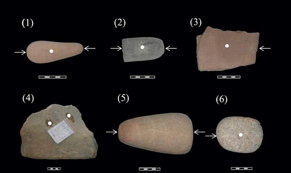
Six ground stone tools of different sizes sit on a black backdrop. White dots and arrows show the parts of each stone that researchers sampled.
Six of the 12 Xincun tools examined for microscopic residues. White dots and arrows show sampling locations. Cropped from Figure 2 to show the first six tools. · Xiaoyan Yang and colleagues · PLOS One, Figure 2 · Creative Commons Attribution · PLOS One

Archaeobotany · 6 min read

Tiny residues on Xincun’s stone tools revealed a palm food

At Xincun, a Late Neolithic settlement on the southern coast of China, excavators processed soil by flotation and recovered no botanical macrofossils. No ancient seeds, fruit fragments or similar plant parts turned up for the researchers to sort. The site had grinding slabs and pestles, implements that gave the team somewhere else to look. In minute cavities on the stones, researchers found two kinds of microscopic remains. Both pointed toward an important food source that could leave very little large debris behind, the soft, starchy interior of a palm trunk.

Xincun sat along the top of a coastal sand dune in what is now Guangdong, southwest of Guangzhou. When the site was excavated in 2008 and 2009 ahead of industrial development, the team uncovered traces of successive occupations over about 8,000 square metres. Occupation layers alternated with deposits of sand. Postholes, hearths, pits and surfaces used by the inhabitants delineated the places where people had lived. Pebble sinkers and other possible fishing gear were among the finds. Dates from charcoal and soot on pottery put the occupations examined by the study broadly in the fourth and third millennia BCE.

The investigators selected 12 ground stone tools from the excavation. Eight were sampled for starch. Four others were sampled for phytoliths. To collect starch, the researchers first cleaned the stones to remove loose dust and used tiny quantities of ultrapure water to wet cavities in the rock. After a few minutes, material loosened from those pockets could be taken up into a pipette. A fraction of a millilitre was enough to bring a sample back to the laboratory. Researchers also examined two sediment samples for starch so they had some evidence about what might occur away from the tools.

Starch is a way for plants to store energy. Inside cells it tends to occur in granules with shapes and internal markings that can be examined with a microscope. Some have layers like the faint contours on a map. In others, the point from which the granule grew is closer to one end and may carry a crack or dimple. A match becomes stronger when several features agree. The investigators compared a set of features with granules from known plants. Their modern reference material drew on collections in China and the United Kingdom.

The starch results included material consistent with edible palms, bananas, freshwater roots and tubers, acorns and a grass known as Job’s tears. Some palm starches resembled ones from fishtail and talipot palms in the reference collection. A single grain matched a reference specimen from another palm, but the authors qualified that identification because they had limited examples from its genus. That difference in confidence is part of what the microscope revealed. It gave the team a good case for palm use, with more tentative identifications for individual palms.

The two sediment samples yielded no starch, whereas the stone samples together yielded 454 granules. The comparison supports an association between the starch and the tools. Two pieces of sediment capture only a little of the ground around an entire settlement. The useful question is whether an explanation can account for several observations at once. Starch was held in pockets on multiple tools, some granules had palm-like forms and a second kind of palm residue appeared on other stones. Each observation adds something the others could miss.

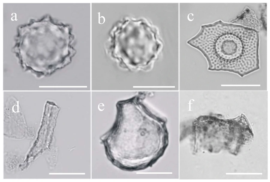
For the phytoliths, the researchers compared material from working faces with material from other surfaces of the sampled stones. A phytolith is a deposit of silica formed within or between plant cells. It can outlast loss of the plant’s organic tissues. The particles attributed to palms in the Xincun study include round bodies with knobbly, sometimes spiny edges. The first two panels of the published micrograph show that outline. Other panels illustrate forms the team attributed to different plants, including a distinctive two-peaked form from a rice husk.

Six microscope images show silica particles labeled a through f. The two images at upper left show rounded palm particles with knobbly edges.
Phytoliths from Xincun tools 9–12. The top-left pair shows palm particles. The lower middle and right show forms attributed to rice. Each white scale bar is 20 micrometres. Resized from Figure 6. · Xiaoyan Yang and colleagues · PLOS One, Figure 6 · Creative Commons Attribution · PLOS One

Palm particles accounted for about 56 percent of the 1,950 phytoliths the team identified. Rice accounted for around one percent. A palm makes silica particles at a rate that can differ from the rate for rice. A tool can also retain some residues more readily than others. These percentages report the mixture the researchers found on four stones. Their importance comes from the combination with the starch evidence. Palm tissues supplied both a recurring silica signature and granules consistent with the presence of useful starch.

The proposal that Xincun people used palms as food draws on what a palm can offer. Certain kinds store abundant starch inside their fibrous trunks. To collect it, people can pound or grate the pith and work it with water to release the starch from the fibers. Settled starch can be collected for use. The method leaves a different set of traces from threshing and cooking grain, where stray pieces of husk and individual seeds can survive in a hearth. Modern starch extraction helps explain how the Xincun evidence could have formed. How the inhabitants used individual tools to prepare the food remains open.

There are layers of inference even in that account. One is that a palm particle reached a stone. Responses to a broader question about diet depend on how much evidence comes from tool use, incidental sediment, or other vegetation nearby. The repeated evidence on tools chosen for their role in pounding and grinding makes food processing a plausible interpretation. Growing the palms close to home, as the authors suggested may have happened, would be a further step. The finds give neither a map of the trees nor a direct measurement of how much of the settlement’s food came from them.

Rice leaves a foothold in the same samples. The team recovered rice phytoliths and considered the available shapes insufficient to establish domestication at Xincun. At another Guangdong site, Gancaoling, later work recovered both charred rice and foxtail millet and identified domesticated rice from the way the grains separated from the stalk. The team there placed early evidence for agriculture at about 4,800 to 4,600 calibrated years before present, roughly 2850 to 2650 BCE. The date ranges from the two sites overlap. The evidence gives the coast more than one story about how people obtained plants during those centuries.

The evidence for Xincun’s food comes in two views. One is of the tools themselves, ordinary abraded stones with the locations of tiny samples marked by dots and arrows. The other is a microscope image in which the palm particles have outlines sharp enough to compare with known plants. Between those views is the laboratory work that made a plant with edible pith visible in a place whose flotation samples offered no identifiable seeds. Which foods come into focus depends on where the investigators look and which tissues they can recognize.

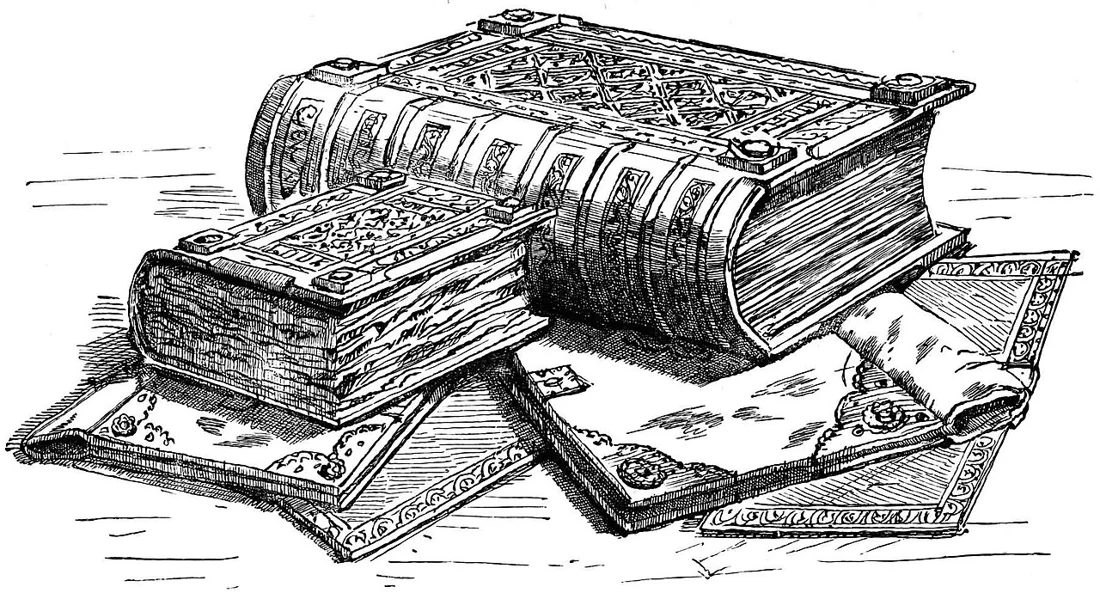
An engraving of thick bound books with decorated covers, a smaller volume, and an open manuscript.
Domesday volumes pictured in William Andrews’s Historic Byways and Highways of Old England (1900). This historical engraving shows an earlier binding presentation, not the books as they are housed today. · Illustration in William Andrews (1900) / Wikimedia Commons · Public domain

History · 5 min read

The smaller Domesday Book kept more of the detail

AI narration · Kaia

Domesday Book sounds like the name of one enormous finished volume. The medieval record actually survives in two principal parts, Great Domesday and Little Domesday. The smaller-format work contains only Essex, Norfolk, and Suffolk, yet its entries often preserve more detail than the larger book. Great Domesday is a condensed presentation of much wider survey material. Little Domesday retains a fuller stage of the process. Their difference gives historians a view of information being turned into a usable instrument of government.

William the Conqueror ordered the survey at Christmas 1085, and the investigation took place in 1086. Twenty years after the Norman Conquest, the king wanted an authoritative account of landed property, its holders, resources, and value. This was a kingdom reorganized by conquest, not a neutral collection of local curiosities. Establishing who held land and what it could yield mattered for revenue and royal power. The record also preserved comparisons with the position before the conquest, making changes in possession and value visible.

The inquiry depended on people as much as on parchment. Royal commissioners held sworn investigations in local courts, asking fixed questions of men who knew the estates and communities concerned. The National Archives describes questions covering the time of Edward the Confessor, the point when a new holder received the land, and the situation at the survey. Officials were therefore gathering information across time and space. Local testimony had to be heard, checked, organized, and carried forward into written returns.

The contents are practical and densely packed. Entries can count plough teams, describe meadow and woodland, record mills, identify classes of tenants, and state values. These details concern the productive and fiscal organization of estates. They do not form a complete register of every individual living in England. Named people are predominantly landholders, while many others appear as totals within categories. Treating Domesday as a modern population census would ask it to do a job for which its questions and structure were not designed.

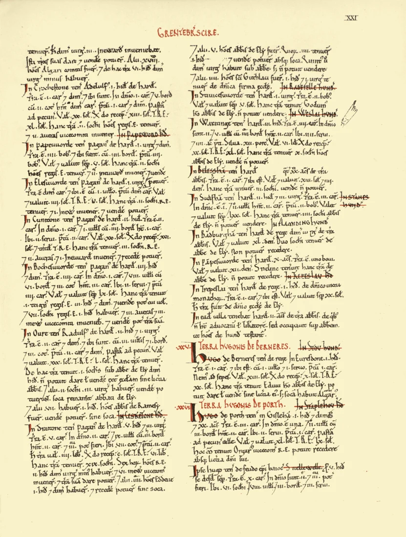
Great Domesday arranged information by county and then by the lands of major holders. Its organization matters: the reader can see a powerful person's holdings together within a county instead of following a simple walking route from village to village. Headings, enlarged initials, and red marks create a hierarchy within the tightly written pages. These are working features, not merely decoration. They help someone find the relevant lord, estate, or entry inside a huge accumulation of names, quantities, and obligations.

A page of the Domesday manuscript with two dense columns of Latin entries and emphasized headings.
A page from the Cambridgeshire section of Great Domesday, cataloged as page 21 in Open Domesday. · Medieval scribe / Open Domesday, via Wikimedia Commons · Public domain

Palaeographers identify most of Great Domesday as the work of one principal scribe. Little Domesday involved several hands and was never reduced to the same concise format. The names Great and Little refer to their physical formats, rather than ranking the richness of every entry. More extensive coverage could be achieved through more aggressive compression. The smaller book consequently gives researchers a closer view of information that may once have existed for other areas before their material was shortened for the larger compilation.

That surviving difference is a reminder that an archive contains decisions about what to keep. A summary can be accurate for its purpose while discarding detail useful to later readers. If a royal administrator needed a compact account of major holdings and value, concision made sense. A historian asking about livestock, local arrangements, or the mechanics of the inquiry may value the fuller return. The same act of editing can make a document easier to consult in one century and less informative for a different question centuries later.

Other manuscripts let researchers investigate those stages. Exon Domesday, preserved at Exeter Cathedral, contains material relating to southwestern counties and survives from the survey process itself. A collaborative study involving Oxford and King's College London examined its scribes, the portions they wrote, and their methods of collaboration. The team's 2021 interpretation described several stages of checking and reorganization, with documents shaped for different fiscal and political purposes. The famous books were outputs of a larger administrative operation, rather than the entire operation preserved intact.

That research also makes the scale of coordination easier to appreciate. Information could be collected in one arrangement and reorganized for another use without electronic storage. The tools were writing materials, trained scribes, ordered gatherings, and shared conventions. Comparing hands and the structure of surviving texts can reveal the work behind the finished page. The researchers' account of a remarkably rapid process rests on those material and textual relationships; it is an interpretation of evidence, not a surviving official schedule that explains every step.

The coverage has important gaps. London and Winchester are absent, as are Durham, Northumberland, and much of northwestern England; some Welsh border areas appear. A place missing from the books was not necessarily uninhabited or insignificant. Absence may concern the scope and survival of the record. Equally, a place that appears under an unfamiliar spelling may be recognizable to local residents today. Domesday joins an administrative landscape of the eleventh century to many locations that still have living communities and changing names.

The physical books have changed too. Their modern binding history means that the two medieval works are now preserved in several bound parts. The engraving shown here records an earlier presentation of the volumes, while the manuscript page reveals the compact written structure beneath the familiar title. A book can remain the same historical work while its covers, division into volumes, housing, and means of consultation change. Digitization adds another way to examine it without making those physical histories disappear.

The surprising value of Little Domesday lies in its difference from the work. It preserves something of the information before the final compression, while Great Domesday shows the power of a disciplined summary. Together they make the survey more than a list of medieval possessions. They reveal a government deciding how to arrange knowledge so it could be used—and leave later readers enough variation to study the decisions themselves.

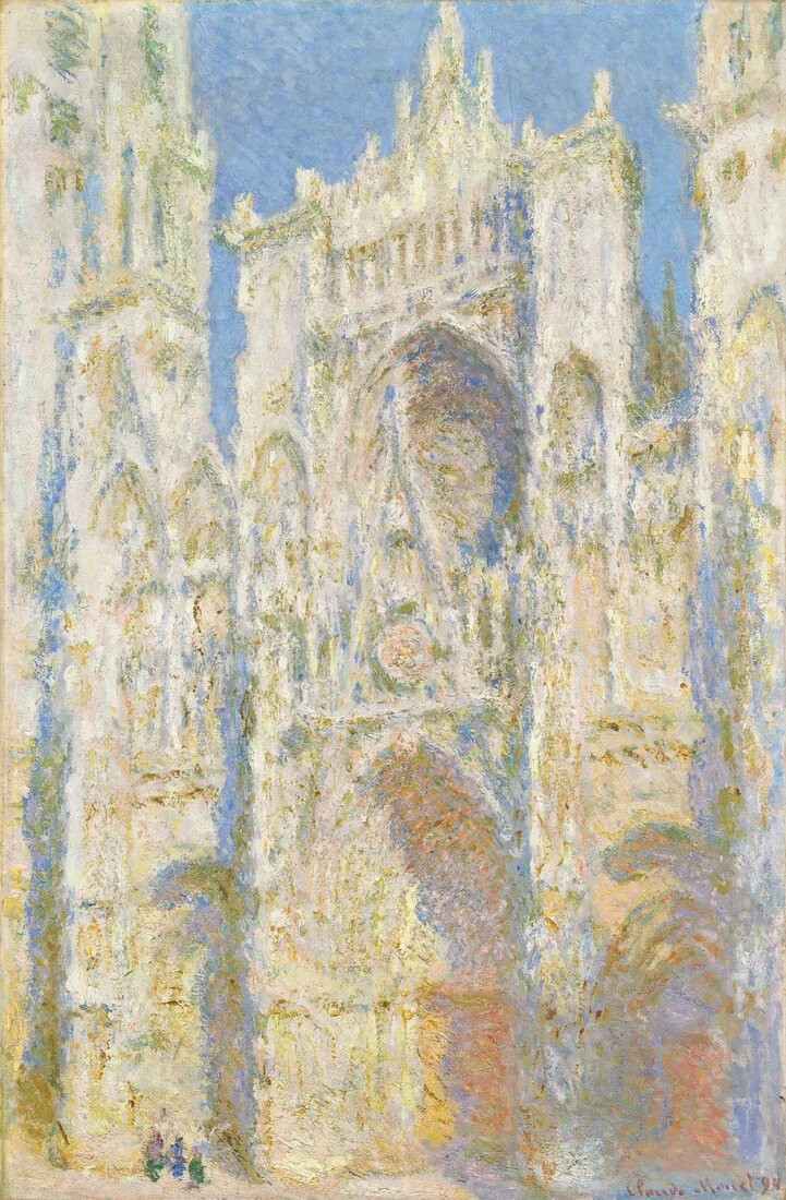
Monet’s cream and gold cathedral façade, with blue recesses and a large pointed portal.
Claude Monet, Rouen Cathedral, West Façade, Sunlight, 1894. Oil on canvas; National Gallery of Art, Chester Dale Collection, 1963.10.179. · Claude Monet / National Gallery of Art · Public domain

Art movements · 5 min read

Monet’s fleeting light took years to finish

AI narration · Fraser

Claude Monet’s Rouen Cathedral paintings look like records of fleeting light. A pale wall flares gold, a doorway sinks into blue, and the stone seems to absorb the air around it. Yet these pictures were not simply finished during the brief conditions they describe. Monet began them in front of the cathedral in 1892 and 1893, then worked on them again at Giverny. Many bear the date 1894. Their apparent immediacy grew through a long process of looking, remembering, comparing, and revising.

That distinction changes the story. The popular image of an Impressionist is a painter rushing to catch a moment before it disappears. There was real urgency in Monet’s work, but urgency was only one stage. The Metropolitan Museum records that he adjusted the cathedral canvases both separately and in relation to one another. A successful picture needed an internal balance. A successful series also needed differences that could be felt across a room. The painted moment was the result of decisions made over time.

Rouen offered an unusually demanding subject. The western front is packed with carved figures, recesses, windows, and projecting stonework. Light does not strike all those surfaces equally. A shallow edge can catch a bright line while a portal remains dark. Atmospheric haze can weaken distinctions across the whole building. Monet rented rooms opposite the façade and worked from windows. He used several viewpoints, so the series is not a controlled set of identical outlines with the colors switched. The architecture anchors an investigation whose conditions keep changing.

Several canvases could be in progress together. When the light moved away from the state he was pursuing on one picture, Monet could turn to another. In a letter of March 18, 1892, discussed by the Musée Marmottan Monet, he reported working on nine canvases that day. That detail suggests both organization and strain. The practical problem was not merely choosing the right pigment. He had to recognize which unfinished image matched the present appearance and recover that picture’s particular relationships before they changed again.

The lead painting, Rouen Cathedral, West Façade, Sunlight, now in the National Gallery of Art, makes a good place to see the result. Its central portal remains legible, but much of the wall is made of small, uneven touches. Cream and warm gold advance against cooler recesses. The main pointed gable cuts into the round window above it. Near the bottom, tiny dark marks suggest people. Their scale helps the wall feel immense even though the view withholds the building’s full height and breadth.

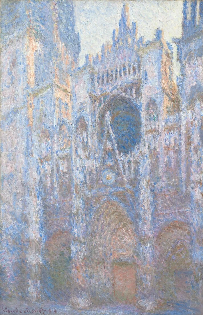
A second Monet cathedral painting with cooler blue passages around the central portal and rose window.
Claude Monet, Rouen Cathedral, West Façade, 1894. A distinct canvas from the series; National Gallery of Art, Chester Dale Collection, 1963.10.49. · Claude Monet / National Gallery of Art · Public domain

The second National Gallery canvas uses a closely related view but gives the façade a different presence. Its cooler blue passages and deeper contrasts gather around the portal and carved edges. The change is not a new architectural discovery: the viewer can still recognize the same nested arches and upward thrust. Instead, familiar stone becomes a way to judge unfamiliar light. Looking between the two pictures makes the stable motif useful. Since the basic subject does not need to be decoded from scratch, differences become conspicuous.

The paint also complicates the idea of a transparent window onto reality. At a distance, patches join into a heavy façade. Up close, they insist on being paint. Their thickness and roughness can echo carved masonry without describing every carved figure. This is a close visual reading, not a claim that each dab records one corresponding stone. The surface lets two experiences coexist: a cathedral that seems to occupy space and a worked canvas whose marks remain visible. Moving between those experiences is part of the pleasure.

Studio revision does not make the original observation irrelevant. It tells us that observation supplied material for a painting rather than an automatic finished product. A color seen outside has to survive beside the other colors placed on the canvas. A bright passage that seemed right in isolation may dominate too strongly when the whole picture is viewed. Revising those relations can strengthen the sensation of a particular light, even when the painter is no longer facing that light. Fidelity can require construction as well as speed.

The series format gave this process another dimension. Monet had already explored repeated subjects, including grainstacks and poplars. At Rouen, the enormous, apparently durable building makes the shifts especially striking. We expect stone to offer permanence. The paintings let its visible appearance become contingent on weather, hour, viewpoint, and handling. This does not mean the cathedral literally loses solidity. It means a viewer cannot separate the experience of the object from the conditions under which it is seen. Repetition makes that dependence unusually easy to notice.

In 1895, twenty cathedral paintings were shown at the Paris gallery of Paul Durand-Ruel. Seeing a group offered something a single image could not: light and color became the relations between pictures as well as qualities within them. A painting could act as a complete work and as one part of a larger argument. The exhibition did not need to reconstruct a precise clock sequence for that effect to operate. The encounter with several distinct versions was enough to unsettle the idea of one definitive appearance.

The useful surprise is the coexistence of patience and immediacy. These paintings can feel fresh because they were carefully worked, not because revision was absent. Their dates, surfaces, and series structure all resist the shortcut of treating them as quick visual notes. Monet returned to the same façade until familiarity became a source of variation. He then returned to the canvases. What looks like a passing instant carries the labor of many other instants, arranged so that we can feel one particular way the world appeared.

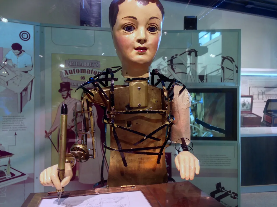
A close view of a seated figure with a painted face and exposed brass framework, a pen in one hand and paper on the desk.
Henri Maillardet’s automaton, made around 1800 according to The Franklin Institute, seen in the museum’s display. The display leaves the brass torso and linkages in view. Resized for display. · Z22 · Maillardet’s automaton at The Franklin Institute (2015), Wikimedia Commons · CC BY-SA 4.0

Mechanical Automata · 6 min read

A writing machine gave its restorers the maker’s name

A mechanical figure arrived in pieces at The Franklin Institute in Philadelphia in 1928. The family that donated it associated it with Johann Nepomuk Maelzel, a name linked to exhibitions of mechanical wonders. Getting the figure to move again was already a considerable job. It had suffered fire damage and gone years without running. When a museum machinist got it working, it bent toward the page, moved a pen, and made a set of drawings and poems. Around a poem it left a clue in French. The writing identified the mechanism as the automaton of Maillardet.

The sheet of paper revealed a name already encoded in metal. Picture a row of brass disks turning in the case under the figure. Their rims have variations in shape, sometimes fine and sometimes broad. A follower bears against a rim and moves as the distance between that rim and the shaft changes. A train of levers and rods can then transmit that small change to the figure’s hand. The curves determined the successive positions that made up the signature. The museum’s repair returned the machine to a condition in which it could put those positions back onto paper.

The Franklin Institute attributes the figure to Henri Maillardet, a Swiss mechanician who worked in London, and dates it to around 1800. Maillardet spent time in the workshops of Pierre Jaquet-Droz, whose business included figures that could write or draw. These were feats of precision engineering exhibited for their ability to perform recognizable human acts in front of an audience. The Institute reports that Maillardet showed his automaton in Britain and traces possible exhibitions farther into Europe. The physical evidence of its writing makes a firmer point than some of the later stories about its travels.

A hand needs more than a single way to move to draw a letter. Give the pen only side-to-side motion and it draws along a line. A second motion at right angles lets it trace a loop across the page. A third motion lifts the pen so the hand can travel between two marks without leaving a streak. The machine has followers for all three directions. Their respective cams turn together, so a lift can coincide with a sideways move, and the pen can descend again where the next mark begins. Those motions have to agree throughout the stroke.

A draft of the pen’s path also has to take into account the hand that actually holds it. The linkages between the cam assembly and the pen pivot and change angles. The maker had to work through that geometry so a movement at the disk became the intended movement on the sheet. Andrew Baron, who later worked directly on the machine, describes 72 closely spaced brass cams involved in encoding the writing and drawing, with additional cams for other movements of the figure. The broad chest below the pen gives the cam assembly and its linkages room to move.

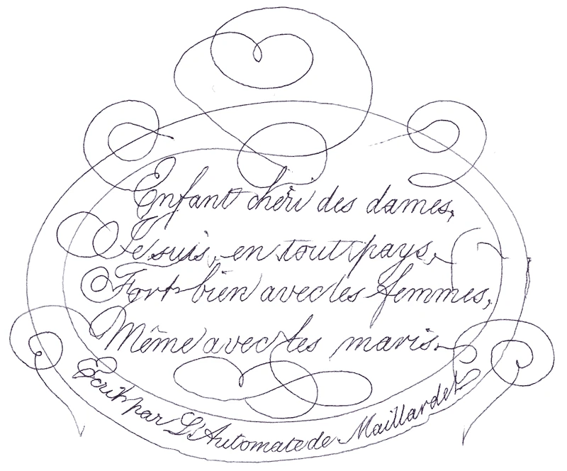
The museum records a repertoire of four drawings and three poems, two in French and one in English. The finished sheets are a second kind of mechanical evidence. The signed French poem shown here contains ornamental lines that sweep around the words and loop back again. Along the bottom edge sits the inscription the Institute transcribes as “Ecrit par L’Automate de Maillardet,” meaning “Written by the Automaton of Maillardet.” The name follows a curve as carefully as the flourishes above it. Each close crossing required the pen to pass through a small area of the sheet on separate journeys. The shape of the cams allowed those lines to meet and part along the same routes the next time the machine performed.

Pen flourishes frame handwritten French verses. A curved line at the bottom names Maillardet’s automaton.
French poem written by Maillardet’s automaton. The maker’s name appears at the right end of the inscription along the bottom curve. Reproduction from The Franklin Institute, converted for display. · Henri Maillardet · Signed French poem produced by the automaton, The Franklin Institute via Wikimedia Commons · Public Domain Mark 1.0

The ink traces also depend on what sits underneath the hand. The original writing instrument is lost, and the Institute reports using a fine ballpoint in its place. Staff also tried a quill and a brush. A different tip can spread ink differently or register a brief touch more or less clearly. A surviving historic impression of one of the drawings shows line qualities that led the museum to suggest an instrument shaped somewhat like a hollow needle. The line on the page brings the path of the hand and the behavior of the chosen tip together.

The automaton’s clothing and some visible body parts have changed as well. The Institute records that the damaged figure was once shown in a long dress, which concealed problems with the legs. Later research uncovered an 1826 lithograph and written descriptions that presented it as a boy. The figure received a new outfit and replacement feet during its exhibition history. In the display pictured here, much of the outer costume has been removed so the structure can be seen. Even an authentic photograph captures a particular state of a long-lived object.

The restorers faced different questions at different times. The museum credits its staff machinist Halsey T. Roberts with returning the machine to working order without its original shop drawings. Later, Joseph Balt took it apart and attended to worn parts. Baron worked on it in 2007 and drew on that earlier repair history. A repaired gear can transmit motion to an old cam. That distinction mattered to the identification. There was enough continuity in the encoded forms for the old curves to produce a name even though the machine around them had needed considerable attention.

Important gaps remain in the object’s route from European exhibitions to the Brock family. The Institute treats possible connections to Maelzel and American showman P. T. Barnum as conjecture. The circumstances of the fire also remain uncertain. The writing sharply narrows the question of who made the machine. The provenance still has to be pieced together from objects, documents and records of appearances. The distinction gives the story its force. A repaired machine can yield excellent evidence about what its maker built into it, while questions about later owners require other records.

The original workshop plans could have offered one path to an attribution. In this case, the linked motions supplied another. To read the clue, the museum needed a mechanism that could turn, a pen, and a flat sheet placed where the hand could reach it. Once these conditions were met the hand followed its old course, lifting at gaps and dropping for the next stroke. The mark that answered the museum’s question came out of the same operation as the drawings and poems the figure had been built to perform.

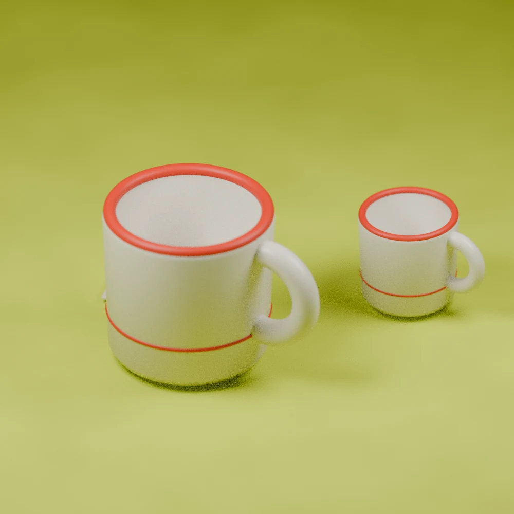
Two modeled cream mugs with fine red bands, a large foreground mug and a smaller distant one on a lime surface.
Original Augustine Atlas still-life illustration of fictional mugs. Their details illustrate the difference between familiarity and precise recall. · Augustine Atlas

Learning & Memory · 5 min read

You can recognize something daily and still struggle to draw it

AI narration · Maeve

A familiar mug can be easy to find in a cupboard and surprisingly difficult to describe after somebody removes it. Was its stripe above the handle or below it? Did the rim carry another line? The object feels thoroughly known because you have used it hundreds of times. Yet using, recognizing, describing, and reconstructing an object make different demands. Research on everyday visual memory shows just how widely those abilities can diverge, even for exceptionally familiar designs.

In a 2015 study, Adam Blake, Meenely Nazarian, and Alan Castel asked people to draw the Apple logo and identify it among alternatives. Only one of eighty-five participants reproduced it correctly, and fewer than half selected the correct version. Participants were often more confident than their performance justified. Confidence was better calibrated when assessed after the drawing attempt. These findings concerned detailed reconstruction and discrimination among similar designs, tasks that ask more than recognizing the brand during ordinary use.

The surprise has a much older counterpart. Raymond Nickerson and Marilyn Adams investigated memory for a United States penny in 1979. Across several experiments, participants struggled with the coin's visual details. Handling a common object repeatedly had supplied ample familiarity without ensuring an accurate account of its arrangement. The researchers interpreted the results in relation to which details are useful in everyday encounters. A coin can be identified and spent without repeatedly inspecting every inscription and its position.

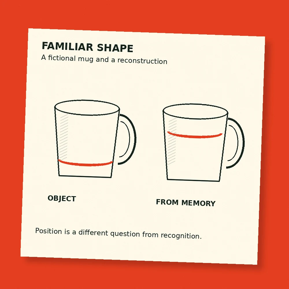
An imaginary example makes that distinction easier to see. Suppose a café serves drinks in cream mugs with a narrow red band near the base. You might recognize yours through its overall shape, the place you left it, or a small chip. When asked to draw the pattern, however, you must specify the band's exact position. The original situation provided several routes to a successful choice. The drawing task removes those routes and demands a particular kind of visual description.

A poor drawing also needs careful interpretation. Someone may remember a shape accurately while finding it difficult to control a pencil. Recognition among alternatives changes the response requirements because the person can select rather than draw. Using both tasks helps researchers separate some of those possibilities. Their questions are about what information participants can demonstrate under particular conditions. A single sketch, taken by itself, would leave more uncertainty about how much difficulty came from memory and how much from drawing.

Visual memory can nevertheless preserve remarkable detail when the task encourages it. Timothy Brady, Talia Konkle, George Alvarez, and Aude Oliva had participants study thousands of object images in a 2008 experiment. Later, people distinguished studied images from alternatives that could differ in fine details, including another example of the same kind of object or a changed state. Performance showed substantial capacity for detailed visual recognition after intentional study. That result describes what people can encode under demanding but structured learning conditions.

A fictional mug is shown beside a partial drawn reconstruction with its red band placed differently.
Original Augustine Atlas comparison. The drawing is an invented example, separate from the published experiments. · Augustine Atlas

The everyday-object studies and the intentional-learning study therefore ask complementary questions. One concerns what survives from ordinary encounters with familiar things. The other concerns the detail retained when people deliberately study many images for a later test. In a kitchen, your goal may be to pour coffee and leave for work. In an experiment, your goal may be to remember what you see. Those goals change which features deserve attention, and the resulting memory should be interpreted alongside the task.

Consider how this matters when giving directions inside a familiar building. You may know exactly where to turn while being unsure how many doors appear along the corridor. Repeatedly following the route has allowed successful movement. Describing every doorway to another person requires a different record. An accurate description can be built by checking the route again with that new purpose in mind. This is an Atlas example of how a familiar environment can support one activity while leaving another surprisingly difficult.

The distinction also matters in design conversations. A customer might recognize a package immediately while recalling its lettering or emblem inaccurately. Asking whether a design feels familiar, whether it can be picked from alternatives, and whether its parts can be reconstructed yields different information. A designer who treats those questions as interchangeable risks answering the wrong one. The relevant test depends on whether the design needs to be found quickly, distinguished from a similar product, or reproduced accurately from memory.

A useful record therefore names the task as well as the result. Saying that a participant recognized a familiar object could mean identifying its general category, selecting the exact version seen earlier, or distinguishing it from a near copy. Those outcomes can differ substantially. Describing the question precisely helps keep an interesting memory result from becoming an oversized claim about everything a person can or cannot remember.

Confidence introduces another layer. Before attempting a drawing, the thought “I see that every day” is easy to produce. It refers to exposure, which is real, but it leaves the precision of the stored detail untested. Trying to specify the arrangement can reveal what that broad feeling leaves unresolved. In everyday work, the useful outcome might be deciding to open the reference image before printing a logo, ordering a matching component, or describing a particular mark to someone else.

None of this requires turning every ordinary object into a study project. A mug can perform its job perfectly while its owner remembers little about the decoration. Detailed memory becomes relevant when a task depends on those details. The interesting discovery is that the feeling of familiarity can remain strong across both situations. It tells us that something belongs to our world, while a more specific question may still require a fresh look at the thing itself.

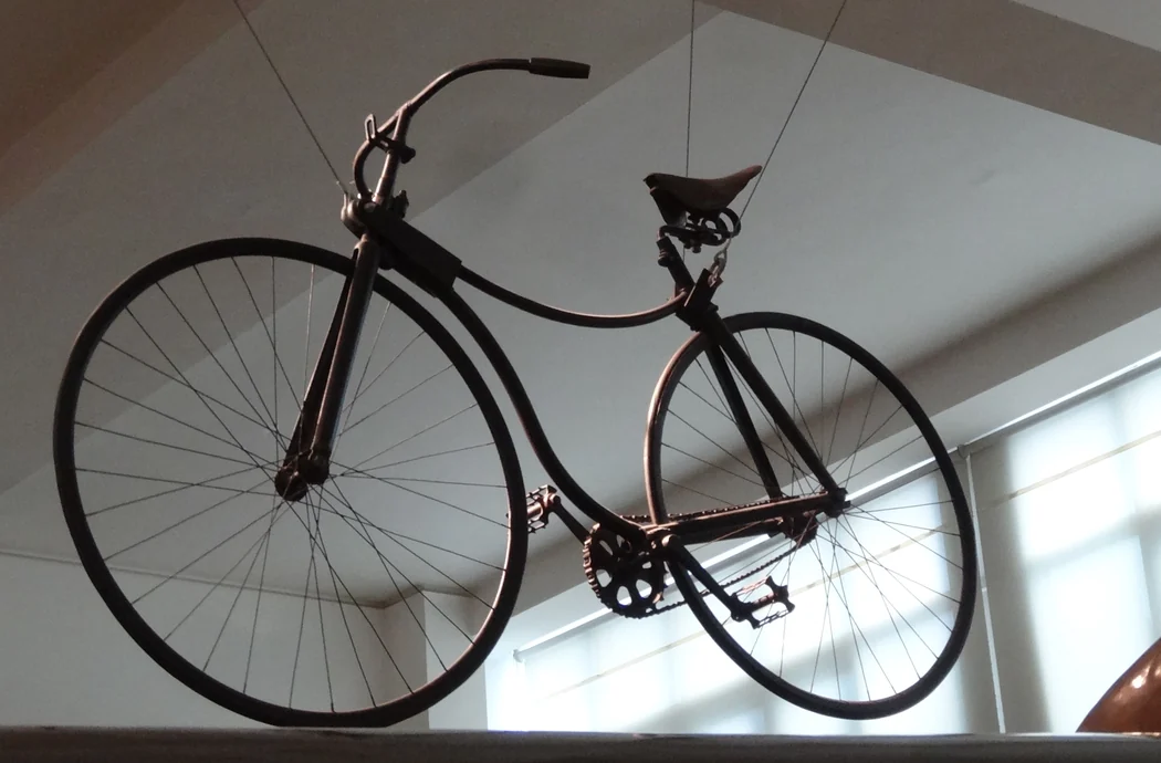
A black 1885 Rover with two similar-sized spoked wheels and an exposed rear chain drive, viewed from below.
The 1885 Rover in the Science Museum, London. Its chain runs to the rear wheel. The museum records that Brooks remade the saddle in 1961. Cropped and resized. · Jonathan Cardy · Wikimedia Commons · CC BY-SA 3.0

Bicycle Mechanics · 6 min read

How the bicycle got its rider down from a giant wheel

In a photograph of the 1885 Rover at London’s Science Museum, the two wheels take up roughly the same amount of space. The saddle sits over the frame, and a chain runs from the cranks to the rear axle. Anyone who has parked a modern bicycle will recognize the layout. Next to a high-wheeler from the same decade, however, the Rover looks almost squat. A change in how the pedals reached the ground made it possible to bring the rider down with them.

On the 1886 Columbia high-wheeler in the Smithsonian’s collection, the pedals turn the giant front wheel directly. The cranks sit at the same axle the wheel spins around. One revolution of the pedals buys one revolution of the wheel. With the same pedaling rhythm, a bigger wheel carries the rider farther on each turn. The easiest way to see it is to imagine two wheels with outside diameters of 30 and 54 inches. One complete turn of the larger wheel covers 80 percent more distance, assuming both roll without slipping. If your feet turn at the same rate on both, the larger wheel carries you 80 percent faster.

A tall machine made that direct drive useful on an open road. The wheel also placed the axle high in the air, and the rider’s feet had to reach cranks spinning around it. A rider typically sat just behind and above the large front wheel, where the legs could reach the pedals and the hands could reach the bars. The much smaller trailing wheel completed the machine and kept its length manageable. In surviving high-wheelers, the relative heights of the cranks and saddle make the rider’s position clear even in an empty museum display.

The arrangement coupled speed to the rider’s ability to manage the machine. It took more than sitting down to get up to the high saddle. A bump or abrupt check at the front wheel could send rider and machine rotating forward. The newspapers collected in the Library of Congress’s guide to the bicycle craze called that fall a header. With the rider’s weight high and near the steering axle, there was little room to move the rider farther back while keeping the cranks within reach. Each gain in distance per pedal turn carried a cost in where the frame put the person.

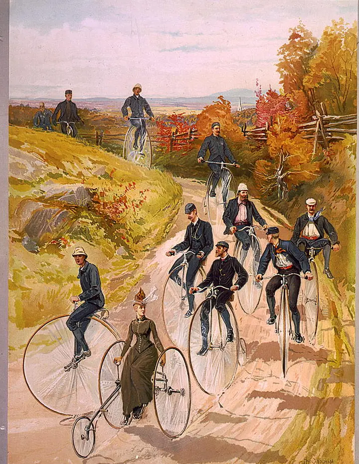
In Henry Sandham’s color print of bicyclists on a country road, published around 1887, several people sit above enormous front wheels. A rider on a tricycle occupies the same road at a different height. The print does something a side elevation in a catalog cannot. It shows how mechanical layouts put bodies into different positions even when the riders are engaged in the same outing. Riders had a reason to endure the height. The bicycle could carry one person a long way under their own power.

An 1887 color print of a group on a country road, including riders seated high above the large front wheels of their bicycles.
Henry Sandham’s print shows riders on high-wheel bicycles alongside a rider on a tricycle. Printed around 1887 by L. Prang & Co. Cropped to the illustrated area. · Henry Sandham and L. Prang & Co. · Library of Congress · No known restrictions on publication · c. 1887

The Rover took advantage of gears connected by a chain. The rider pedaled around one axle while the chain turned a small sprocket around a second axle. A full turn of the larger front chainring pulled enough chain to make the smaller rear sprocket turn more than once. As long as the connection was engaged, the rear wheel turned at that faster rate. The front wheel could now steer with its own fork without also sharing its axle with the cranks. The designer could decide how far the machine traveled per turn separately from how high to mount the pedals.

For a simple comparison, suppose a high-wheeler has a 54-inch driving wheel. Give another bike a rear wheel 27 inches across and arrange its chain drive so the rear wheel turns twice per crank turn. Each machine now rolls the same distance per turn of the cranks, about 4.3 meters. The 27-inch example is a comparison, with round numbers, of how the layout works. On the museum Rover, the visible chain drive works on the same principle. The wheel can be smaller because it can turn more often than the pedals.

John Kemp Starley’s 1885 Rover is the model the Science Museum identifies as the first successful safety bicycle. Designers had already been working on ways to lower the rider during the preceding decade. The early Rover is recognizable as a relative of today’s bicycles even though its curved frame tubes and solid rubber tires belong to an earlier era. Its power goes to the rear wheel, its front wheel handles steering, and its saddle and cranks sit within the small space between two comparatively modest wheels.

The name safety bicycle described a change in how someone could use the machine. Bringing the saddle lower and placing more of the rider between the wheels reduced the tall machine’s particular tendency to pitch a rider over the front. Getting underway no longer required climbing to a saddle perched high over the driving wheel. Other parts also mattered to how any individual bicycle handled, including braking, steering geometry and the distance between the wheels. The Rover’s contribution was to give designers room to change those features without taking away the rollout riders valued.

The shift also shows up in manufacturing. The Smithsonian’s record of the Columbia notes that the Pope Manufacturing Company sold high-wheelers in the 1880s and later sold Columbia safety bicycles in the 1890s. Its overview dates the introduction of a Pope safety model to 1888 and the end of its high-wheel production to 1892. The two layouts coexisted for a while. Looking at an 1887 cycling book such as A. J. Wilson’s makes the overlap visible. The ordinary roadster and the Rover each merited an illustration, and a reader could compare their profiles on paper. Even without riders in those illustrations, the height of the two saddles above their respective cranks gives away what mounting each bicycle involves.

An early Rover still carries a great deal of the old bicycle in its form. It has slender metal spokes and a wheel built to travel along rough roads. What changed was the relationship between a slow set of turns at the pedals and a faster set of turns at the driving wheel. In the giant front wheel, speed and seat height had partly been consequences of the same choice. In the Rover, the chain let designers choose them separately. That is the mechanical idea preserved in the familiar sight of a rider stopping on a modern bicycle with a foot close to the ground.

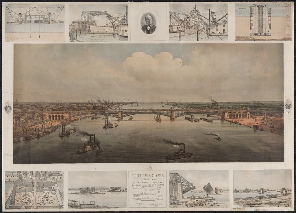
A color print of the St. Louis bridge over the Mississippi, framed by smaller construction scenes and a portrait.
The St. Louis bridge as depicted in an 1874 chromolithograph based on photographs by R. Benecke. The smaller scenes track stages of construction. Resized for display. · F. Welcker · Based on R. Benecke photographs · Library of Congress · Public domain in the U.S. · Published in 1874

Bridge Engineering · 6 min read

The crew tried 60,000 pounds of ice to close the Eads Bridge arch

In September 1873, the builders of the Eads Bridge in St. Louis had to join steel arch ribs over the Mississippi. Henry Flad, the assistant engineer in charge on site, tried cooling the metal with ice. According to the Historic American Engineering Record, the crew started with 15,000 pounds and went through a total of 60,000 pounds. The parts still would not go together as intended. The crew made the connection using a wrought iron plug, following a change James Eads had recommended. The ice belonged to a real engineering problem. At the end of a long steel frame, a modest movement could decide whether the pieces came together.

The bridge was designed around three large steel arch spans over the river. Their curved ribs would carry forces toward the masonry supports. The curve gives a downward load a route toward both ends, where the supports resist an outward thrust as well as a vertical reaction. Each rib had to be joined across the opening before it could do that work as a continuous arch. Until then, the two advancing halves had free ends over water. A structurally useful shape on the finished bridge could be precarious in the middle of construction.

One way to erect an arch is to build a temporary supporting frame below it. The pieces rest on that frame until they connect and can transmit load through the arch to its permanent supports. That temporary construction is known as falsework. In St. Louis, piers and supports filling the channel would have interfered with steamboats. Keeping the river open shaped the type of construction the engineers could use. They concentrated the temporary equipment up on the piers and abutments, then supported the new steelwork with cables from above.

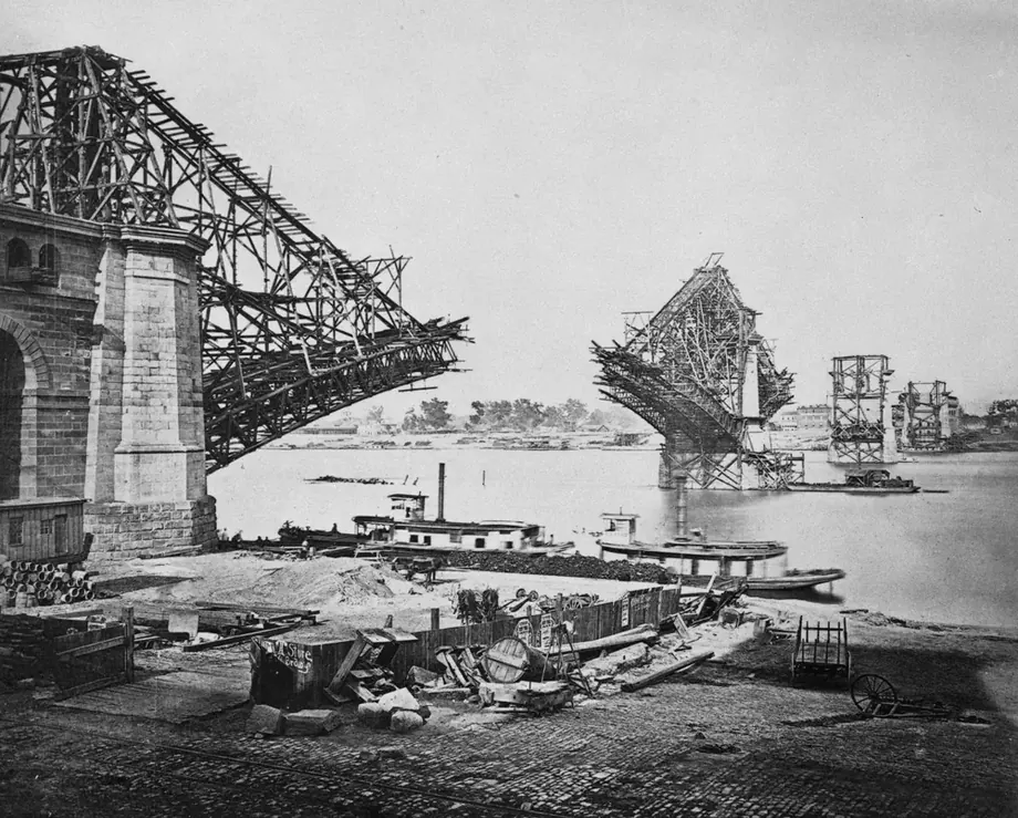
The arrangement included temporary timber towers and a rig that balanced the work as it projected out over the water. The builders could extend a half arch in stages and hold its growing weight with a set of attachments. The cables pulled upward on the rib where they attached and passed the force back to the temporary rig. A change in an attachment or the amount of tension could move the rib. Jacks let the crew adjust the rigging as conditions changed. In effect the engineers had to design and manage a second structure that would live only long enough for the bridge to stand on its own.

In Woodward’s photograph of the west arch work, the steel curves out into the opening beneath cables that stretch up toward the temporary tower. The photograph dates from construction and was reproduced in his 1881 book. Woodward identifies the numbered joints reached by two of the cables. The diagonal lines through the sky explain what supports the steel at that moment. Their eventual removal would make the completed crossing look simpler than the structure the crews had needed to assemble it.

Two incomplete arch halves project toward each other over the river, with temporary timber structures and cables above them.
West arch erection, reproduced as Plate XLII in C. M. Woodward’s 1881 account. The construction cables shown reach joints 6 and 9. Cropped to the construction photograph. · C. M. Woodward, 1881 · Historic American Engineering Record MO-12-96 · Library of Congress · Public domain in the U.S. · Published in 1881

The west span was approaching closure on September 14. The archival report places Eads in London, where he was negotiating a loan that depended on the arch closing within five days. Flad had to manage the steel and rigging in St. Louis. The record notes an air temperature of 98 °F late in the afternoon on September 16. The metal structure and its support cables responded to their own temperatures. Heating could lengthen one piece more than another and change the alignment where the two ends approached. Lowering the temperature with ice was an attempt to bring pieces back into a position where they could be joined.

The scale makes the attempt understandable. A free steel bar 100 meters long can lengthen roughly 12 millimeters when the steel warms uniformly by 10 °C. That is an illustrative calculation for a straight bar. On the Eads project, several connected members and cables warmed by varying amounts, and some were restrained. The resulting movement at the connection depended on their angles, lengths and supports. An end could sit too high or too low as well as too close or too far away. A crew could spend hours adjusting the rig and discover that its target position had shifted in the meantime.

The ice did not produce a fit. The HAER account says Flad adopted Eads’s recommendation to shorten the last arch members at their ends and use a bolted, wrought iron plug to link them. The western closure described in the report was made by 10 p.m. on September 17. The crew’s new connection gave the structure a way to join within the conditions it actually faced that night. A message reached Eads the next morning and the loan was secured. Work continued on the other ribs and spans, with the inner ribs of the center and east arches linked by December.

Closing a rib changed how loads could travel. It also left a transition to manage while the temporary gear stayed in place. In January 1874 Theodore Cooper, the chief inspector, found two ruptured tubes. With Flad ill and Eads away in New York, Cooper sent word by telegraph. According to the HAER account, Eads responded with directions to reduce strain from the construction cables that still remained. Replacement tubes were installed. The report describes no further construction trouble of that kind once the temporary cables were removed. Forces present after the plug went in could still depend on how much load the rigging was holding.

A public load test in July 1874 gave the arches a very different assignment. Fourteen locomotives and their tenders supplied a reported 700 tons. The engineers brought them across the rail deck in different arrangements, including two groups of seven that used both tracks and stopped at the middle of the bridge. By then the load could travel through the connected ribs. The goal was to observe the completed crossing under a deliberately heavy load in positions that the test crew could choose.

The bridge was formally dedicated two days after the test. In an earlier stage shown in Woodward’s Plate XLV, the ribs are continuous and the roadways are under construction above. The connected ribs could support the rest of the structure through the masonry supports. The surviving construction images tell two stages of the same story. In one, cables and towers are essential to the visible steelwork. In the other, the arches have become a path for weight over the Mississippi. What the crew had to solve on that hot September day was the small, stubborn connection that let the steel begin to change from one system to the other.

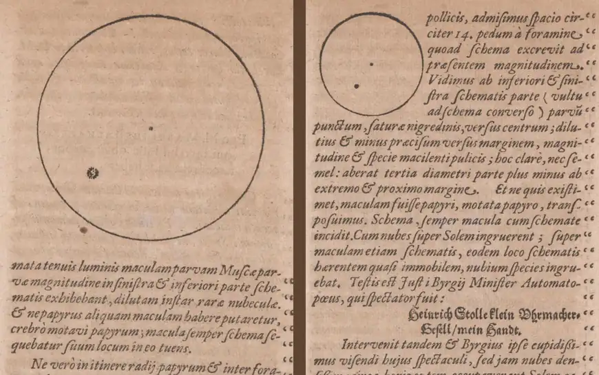
Two crops of printed pages show outlined solar disks, each with a dark spot in its lower left quadrant. The left circle is larger in print.
Two solar drawings from Kepler’s 1609 account of his observations in Prague. The larger disk is from his home and the smaller disk from Bürgi’s workshop. Cropped from separate pages, placed side by side and lightly smoothed for display. · Johannes Kepler · Phaenomenon singulare seu Mercurius in Sole (1609), fols. D2r and D3r, ETH-Bibliothek Zürich, Rar 4342: 5 · Public Domain Mark 1.0

Camera Obscura · 6 min read

Kepler thought he saw Mercury. His drawings recorded a sunspot.

On May 28, 1607, Johannes Kepler went looking for Mercury. He thought the planet might cross in front of the Sun and appear as a small dark silhouette. From a darkened room in Prague, he used a camera obscura to cast the Sun onto paper. He found a dark mark against the bright disk and recorded where it was. He later published his account with diagrams and called the event a passage of Mercury. The mark was a sunspot group. A study published in 2024 showed how the drawings could help date a solar cycle more than four centuries later.

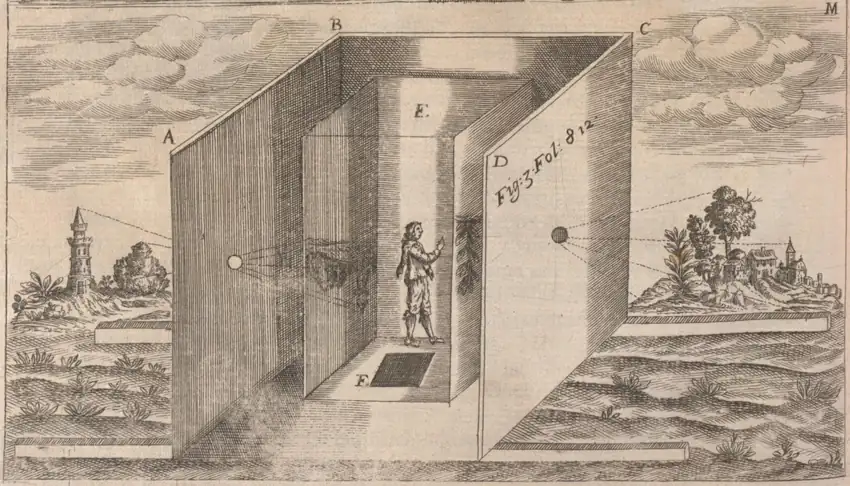
The observing chamber mattered because sunlight could be put onto a surface with a position and a scale. Kepler used a small opening to send the solar image across the dark interior. The edge of the disk provided a boundary. A mark near one part of that boundary had a position that could be sketched and compared with a later view. The small opening inverted the image. That optical fact became important to later researchers because it affected how they read the relative positions of the disk and the mark. They also needed to distinguish the orientation of the image from the orientation of the printed page.

Kepler made an observation at his home and another at the workshop of the Swiss clockmaker and mathematician Jost Bürgi. His account gave readers details about the afternoon, including a reading of Prague’s astronomical clock as he passed through the city and the approach of sunset during the second observation. The clock reckoned time from the previous sunset. That system is unfamiliar now, but the note gives researchers a way to estimate when Kepler reached each observing site. A fact about a walk between buildings ended up helping fix an astronomical image in time.

At home, Kepler shifted the receiving paper repeatedly. A mark on the sheet itself would move with the paper, whereas the mark he was investigating kept its position relative to the projected disk. At Bürgi’s workshop, he describes the paper receiving the image at a distance of about fourteen feet from the opening. There, too, he moved the paper and saw the mark stay with the disk. Those checks made a defect on the receiving surface a less plausible explanation. The question of what had made a real mark in the solar image remained open.

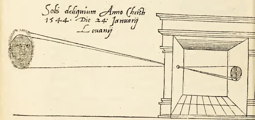
Solar projection was already a documented method. In Leuven on January 24, 1544, the mathematician and instrument maker Gemma Frisius observed a solar eclipse. The book he published the following year shows the solar disk at the left of a woodcut and a small building at the right. Lines lead toward an opening in the dark chamber, cross and reach the interior. The print presents the room, the aperture and the receiving surface as parts of one apparatus. A reader could understand the arrangement from the image and use the surrounding instructions to make sense of what appeared.

Frisius also gave the image a scale. His text describes dividing the diameter of the Sun into twelve equal parts with a compass, then using those divisions to estimate the extent of the eclipse. He reported a little more than ten of those parts, conventionally called digits. Those divisions ran along the diameter. They expressed how far the eclipse extended across the disk, which is a different quantity from the fraction of its area covered. He also called attention to the side of the projected disk that darkened. Because the rays cross at the opening, an event high on the Sun appears low in the chamber.

A 1545 woodcut shows the eclipsed Sun at left and two lines of light crossing at the hole of a small building. A circle marks the projection inside.
Gemma Frisius illustrated the dark chamber he described when reporting the 1544 solar eclipse in Leuven. Cropped and resized from the original volume scan. · Gemma Frisius · De radio astronomico & geometrico liber (1545), John Carter Brown Library · Public Domain Mark 1.0

A dark patch in the projected Sun can have several causes. Frisius knew he was observing the edge of the Moon as it crossed the solar disk. Kepler saw a much smaller mark and identified it as the silhouette of a planet. Sunspots are darker regions of the visible solar surface associated with strong magnetic fields. In a small or indistinct projection, a group can register as a single dark patch. The instrument preserved the location of the light and dark regions on paper. The identity of the thing responsible still had to come from other evidence about how it moved, what it looked like and what could have been in the line of sight.

Hisashi Hayakawa and colleagues revisited the 1607 observations in the twenty-first century. Their problem was to say where on the Sun the recorded spot lay. The angle of the Sun’s equator as seen from Prague depends on when the observer looked. A position described as high or low in a room refers to the local vertical. The researchers had to convert Kepler’s views to solar coordinates before comparing them with later records. They used clues from the account to estimate the places and times, then calculated the orientation of the Sun at those moments.

The two full-disk sketches show the mark in somewhat different positions. The early projection, the original hand drawing and uncertainty about the viewing times all affect the precision of a reconstruction. Nevertheless, both observations placed the spot group near the solar equator once the researchers accounted for the image orientation. They compared those low latitudes with later observations. The first telescopic records from the 1610s include sunspot groups at higher latitudes, a pattern the researchers could use to place Kepler’s group in a longer sequence.

Sunspot groups generally appear at higher solar latitudes early in a cycle. As the cycle advances, the zones where new groups appear move toward the equator. The position of a group gives some evidence about the stage of its cycle, even when a continuous tally is unavailable. On that basis, the researchers judged that the group probably belonged to the cycle ending around the time of Kepler’s observation. They placed the start of the following cycle between his sketches in 1607 and the emergence of telescopic records in 1610.

That timing matters to comparisons with other ways of estimating past solar activity. Observers today can build a record from successive views. For earlier centuries, studies may also turn to indirect evidence, including radiocarbon levels in dated tree rings. Different reconstructions have implied different cycle lengths around the early 1600s. A low-latitude group in 1607 provides a separate observation to compare with them. Its value comes partly from falling in a gap just before a more extensive record began.

Frisius’s woodcut shows why a report about the Sun sometimes needs a picture of a building. Kepler’s drawings show why it sometimes needs a note about a city clock. The modern analysis depended on the conditions under which the marks were made. The edge of the solar disk and a location within it survived in the drawing. His account of the afternoon put the drawing in context. Kepler gave the dark spot the wrong name. He preserved enough of what he saw for someone centuries later to place it in the history of the Sun.

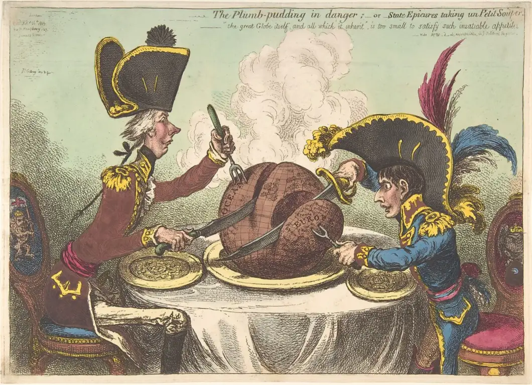
Pitt and Napoleon, in uniforms and oversized hats, carve a steaming globe at a table set for two.
James Gillray, The Plumb-Pudding in Danger, February 26, 1805. Pitt cuts into the Atlantic at left, while Napoleon’s fork holds the piece marked Europe. Museum scan resized for display. · James Gillray, published by Hannah Humphrey · The Metropolitan Museum of Art, 42.121(93) · Public domain · The Met Open Access

Caricature · 6 min read

Gillray made the world a pudding for two rival leaders

Steam rises from the globe in James Gillray’s hand-colored etching The Plumb-Pudding in Danger. At first it looks like a rich, dark pudding served on a large plate. On a closer look there are lines of latitude and longitude on the crust. The word Europe is visible on the slice at the right. At the left, British prime minister William Pitt has already cut deep into the other side. His rival, French emperor Napoleon Bonaparte, digs in with tools of his own. Gillray put two states at war into the familiar arrangement of a dinner for two.

The print appeared in London on February 26, 1805. Britain and France had resumed war in 1803 after the Peace of Amiens broke down. Napoleon became emperor in 1804, the same year Pitt returned as prime minister. Napoleon and Pitt were recognizable figures to the London audience for Gillray’s prints. Their uniforms and sharply different outlines help place them even before the viewer identifies the maps. Both have high collars, bright metal trim, and enormous hats. Behind their chairs are heraldic signs. Their details add to the sense of an official dinner, even as the great hats make it seem absurd.

Pitt’s position makes his work look almost methodical. His profile comes close to a vertical line from his hat to his coat, although his near arm and knife extend far into the picture. He drives a trident-like fork into the globe and draws a long blade across it. The British Museum identifies his portion as the Atlantic, including the lucrative West Indies. The reason for the unusual fork becomes clearer with that geography in mind. The utensil is part of the joke about naval power, giving Pitt a means to hold the ocean steady while the knife does its work.

Napoleon’s posture gives his side a different rhythm. He rises to reach the table and brandishes a blade that reads as a sword. The stamp of Europe on his wedge is plain when the eye traces that blade. The British Museum points out that his fork goes into Hanover, a German territory linked to George III. An intricate diplomatic and military rivalry becomes a nearly instant contrast of shapes. Pitt cuts a wide ocean portion while Napoleon bears in toward Europe. A reader can grasp the distribution even when the smaller place names on the map are too tiny to make out.

A pudding can be divided into servings from an apparently ownerless center. Treating the globe that way is part of Gillray’s argument. The world’s inhabitants would have made very different claims on the territory that he labels on this serving dish. They have no place settings in the drawing. Just two diners have plates, seats, and utensils. That restriction gives the satire its force. It encourages a viewer to notice whose interests the men appear to have in mind while making the positions of everybody affected almost disappear. The print presents a British caricaturist’s argument about power and appetite.

There is also an important symmetry in the setup. Many of the print’s readers in wartime London could have been ready to laugh at Napoleon. Gillray gives them the small emperor, but sets Pitt’s utensils against the same meal. The apparent ease of Pitt’s reach can look more calculating than Napoleon’s effort. Both are intent on securing their portion. The comparison carries the criticism farther than a picture of one enemy grabbing too much. It makes the behavior intelligible as something two rivals share, even though their tools and their parts of the map differ.

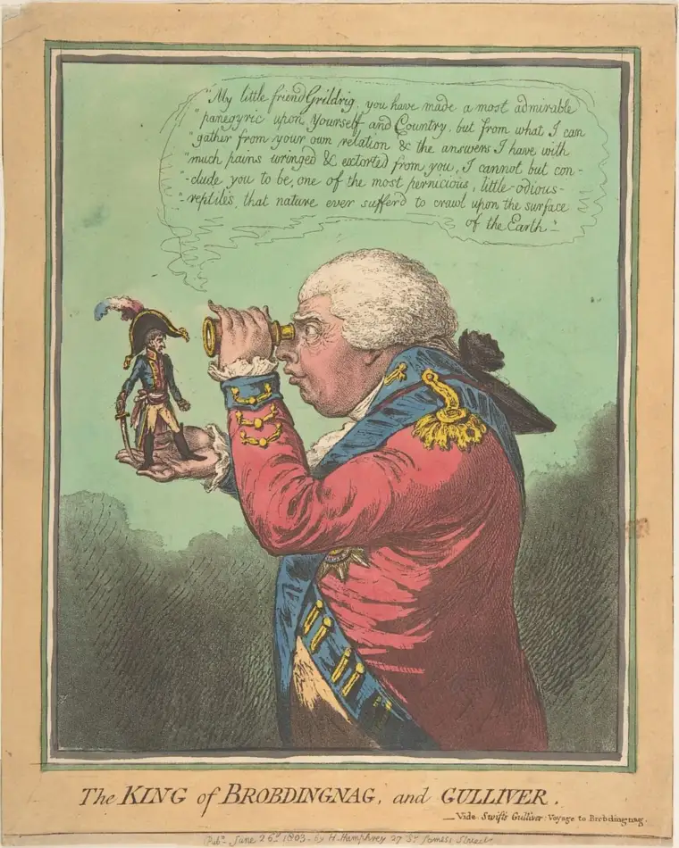
Two years earlier, Gillray had put a much smaller Napoleon in a different set of hands. In The King of Brobdingnag and Gulliver, George III holds him up and studies him through a spyglass. The print appeared in June 1803, only weeks after the breakdown of peace. The giant king comes from Jonathan Swift’s tale of the country of Brobdingnag. Swift’s king asks Gulliver to explain his homeland and is dismayed by much of what he hears. In the print, the British king takes the position of the large spectator and the French leader becomes the little visitor whose braggadocio is under examination.
A towering George III peers through a spyglass at a miniature Napoleon standing in his hand.
Gillray’s King of Brobdingnag and Gulliver, June 26, 1803. George III examines Napoleon as if he were a tiny visitor from Jonathan Swift’s novel. Museum scan resized for display. · James Gillray, after Thomas Braddyll, published by Hannah Humphrey · The Metropolitan Museum of Art, 17.3.888-313 · Public domain · The Met Open Access

That earlier caricature puts a threat inside what first appears to be a reassuring arrangement. Napoleon is small enough to fit in a palm, and the king needs an instrument to examine him. The little figure still stands with an unsheathed sword. The Met connects that hint of danger to contemporary fear of a French invasion. Size works as a political judgment inside the drawing. A large king lends confidence to the scene, while the visible little weapon calls the confidence into question. Two years later, the great hat and small body are again close together. The setting has changed, and now Napoleon’s blade cuts a piece of the world.

Both prints bear the name of their London publisher, Hannah Humphrey. Their details reward the kind of close examination a print allows. From across a room the long blades and the globular meal give the later picture an unmistakable structure. At reading distance the words on the globe and the emblems on the chairs identify what the people and objects stand for. The medium also matters to the experience. Fine etched lines describe crosshatching, utensils, and cloth, while color helps the eye separate the two sets of clothes and pick out the bright decoration on each hat.

The engraved subtitle calls the diners state epicures out for a small supper. The joke needs very little translation. A supper described as small takes up the whole table, and its main dish contains the known world. Even the steam helps Gillray make the idea work. It is high and pale enough to hold the space between the two hats, and it gives a map the physical warmth of something just carried to the table. A globe sits on a stand in the room of a geographer. This one comes on a serving plate with two smaller plates ready beside it.

A political picture can simplify so elegantly that its interpretation feels like something that simply happened. Here the place to keep both in view is the seam in the pudding. It shows what Gillray wants his audience to think about. Each diner acts as though the land and sea in front of him can simply be portioned off. The surviving 1805 print provides evidence of how a London caricaturist made a war legible to readers. Its table remains an invented place, shaped to turn policy into an appetite that anybody who has reached across for a second helping can recognize.

Dark Shang bronze cauldron on three legs with two upright handles and a fine vertical ridge through the animal face on its bowl.
The tripod cauldron of Ran, late Shang dynasty. A shallow ridge bisects the raised mask and records a division in the mold assembly. Museum photograph cropped with the studio backdrop extended at the sides. · Art Institute of Chicago · Tripod Cauldron of Ran (Ran ding), Lucy Maud Buckingham Collection, 1928.167 · Public domain · Art Institute of Chicago image via The Last Museum

Metal Casting · 6 min read

A Shang bronze cauldron wears the joints of its mold

A narrow ridge runs down the animal face on a Shang bronze cauldron in the Art Institute of Chicago. On either side, raised eyes and horns stand clear of a ground crowded with small angular spirals. The ridge is low enough to pass for another stroke in the pattern. The museum identifies it as the place where sections of the clay mold came together. Whoever planned the surface made the line through the face do two jobs. It belongs to the vessel’s symmetry and it preserves evidence of how the bronze took shape.

The bowl stands on three legs and has two upright handles at the rim. Vessels of this family are called ding. In Shang ritual life, a bronze vessel could hold food offered to ancestors and belonged to a system in which the type and display of vessels conveyed rank. The museum’s example, cataloged as the tripod cauldron of Ran, is about 24 centimeters high with its handles. The face occupies a band on the outside of the bowl. Another mark appears inside, where the collection label identifies a cast family emblem called Bing. The two kinds of marks belong to the same vessel and tell different parts of its history.

A piece mold has outer sections that fit together to define the exterior of a casting. A vessel also needs an inner boundary. In descriptions of ancient Chinese bronze production, a clay core occupies the bowl’s interior, leaving room for metal in the space between it and the outer sections. The outer sections can carry impressions taken from a model and details worked into the clay. Once assembled, they enclose a gap with the depth and contours of the walls that will survive. A raised eye on the metal corresponds to a recessed feature in the surface facing the metal.

The outside of a round vessel presents a design problem. You can follow the pattern around the curve, yet a maker working with sections had to think about where a surface would end and begin again. A tiny change where clay faces meet may show in metal. On the Ran cauldron the meeting line sits at the axis of the ornament. Horns, eyes and curls give the eye something to follow on each side. The division reads as part of the composition even before you learn that it corresponds to the assembly of the mold.

The arrangement belongs to a broader tradition of carefully balanced decoration. The Metropolitan Museum of Art’s study of the Morse collection describes vessels whose designs occupy areas defined by sections of a mold. Other surfaces build tiers of decoration around recurring vertical axes. Similar habits of symmetry appear in Shang designs in materials that are worked in other ways, including stone and jade. The pattern on one vessel therefore carries evidence about the shape of the mold alongside choices that artists in several materials could share.

Actual pieces of used molds offer a way to investigate the work from the clay side. A research team examined a decorated sherd from Daxinzhuang, an archaeological site in what is now Shandong, to the east of the late Shang capital near Anyang. Its traces were measured with several methods, including X-ray tomography, which revealed pores inside the clay. The researchers proposed that the pores helped air move through the mold and concluded from the material analysis that the fragment was made locally and used for bronze casting. The excavation gives it a place and context that a visible line on an old collection bronze alone could rarely supply.

Six views of an excavated clay mold fragment from Daxinzhuang, including its patterned face and a centimeter scale.
A clay casting-mold fragment recovered at Daxinzhuang, east of Anyang. The fragment comes from a separate site and documents how similar casting work survives in clay. Published figure adapted for display. · Yunbing Zong and colleagues · Daxinzhuang casting mold sherd, PLOS ONE, Figure 2 · CC BY 4.0 · PLOS ONE

The pattern on the sherd is small enough to hold close in the photograph. Marks and boundaries that would rise from gold-colored metal on a finished vessel appear against a rough clay surface. The sherd can be studied as a tool in its own right. The researchers examined how the decorative profile related to the clay around and beneath it and interpreted the material as evidence that the pattern on this fragment was carved. A bronze photograph offers a clearer impression of the overall design, while a fragment preserves some of the decisions that let the design pass into metal.

The Daxinzhuang team dated a pig bone from the same excavation unit and used the result to place the sherd around the transition from late Shang to early Western Zhou. That association supplies an approximate date for the fragment. It is also a reminder that a fragment of a mold and a complete vessel need independent evidence before anyone can link them. In this case, the curve and the decorated inner face were among the reasons to identify the sherd as part of a vessel mold. The excavation context helps place the workshop evidence in time.

At the Xindian site in Anyang, Shirui Lin and colleagues studied a larger group of late Shang mold materials and found several deliberately different clay preparations. The researchers distinguished materials used for different parts of an assembly and found evidence for different firing histories in outer mold pieces and inner cores. They also identified coatings that seem to have served different tasks at contact surfaces. Their results give substance to the word “fit.” It involved the behavior of several prepared materials as well as whether the shapes of two pieces would line up.

A bronze’s current surface can also reflect events much later than its manufacture. The Art Institute describes the Ran cauldron’s original metal color as golden. Burial changed the surface, and the museum reports that the object was later cleaned, recoated and darkened, probably by heating. Its present blackish brown has a history of its own. The prominent eyes and the narrow vertical division survive that history. Their shapes can still be followed across shadows on the dark surface. Color alone would leave the original sheen much harder to recover.

It is possible to read more than one kind of intention from the finished bowl. The inside emblem supplied a name or group identification in the vessel’s own cultural setting. The outside faces organized a great deal of decoration into a repeatable pattern around a curved wall. The flange made the arrangement of that pattern legible and let a feature of the mold remain in view. The excavated fragments and the finished bowl preserve different views of how those working surfaces met. A thin strip of bronze lets that evidence stay visible in the finished design.

A printed folding table pairs Memory, Reason and Imagination with History, Philosophy and Fine Arts, then breaks the History and Philosophy divisions into numbered chapters.
Foldout classification table from the 1815 Catalogue of the Library of the United States, prepared by George Watterston. University of Michigan copy digitized by Google via Internet Archive. Rotated for legibility and cropped to the table. · University of Michigan copy · Google scan via Internet Archive · Public-domain 1815 publication · Library of Congress item and rights information

Library Classification · 6 min read

The 1815 Library of Congress catalog put an alphabet inside Jefferson’s subjects

Open the 1815 Catalogue of the Library of the United States at its first chapter and the page gives you three instructions. It says you are in Memory, then in civil history, then in ancient history. Below that stack of subjects, the entries start with three French abridgments under A, followed by works entered under Aelian and Ammianus. The subject map came from Thomas Jefferson. The alphabetical sequence below the headings reflects a decision by librarian George Watterston. Look from the printed foldout to that opening page and you can see the two forms of order together.

Congress bought Jefferson’s library in 1815, and Watterston prepared a printed catalogue for the new congressional collection. A contents page helps a reader jump directly to a chapter. The foldout goes further by showing the relationships among chapters. Its table describes the faculties of the mind and matches them with fields of knowledge. Memory corresponds to History, Reason to Philosophy, and Imagination to Fine Arts. The large divisions tell you where a field fits. The chapter numbers connect that idea to the way the catalog can actually be used.

From the History branch on the foldout, trace the civil line to Chapter 1 for ancient history, then to modern history divided into foreign, British and American chapters. Follow the natural line and you find physics and agriculture, as well as the branch with plants and minerals. Watterston retained this high-level subject grouping. Its pattern follows the system that Jefferson explained in his May 1815 letter to the librarian. Jefferson started with Francis Bacon’s account of human knowledge and adjusted it for use with the range of books he owned.

The printed table makes those groupings unusually visible. Memory stretches across branches of civil, ecclesiastical and natural history. The chapter dealing with botany sits in that last branch. Someone opening a present-day library guide might expect botany under science. In the 1815 catalogue its place reflects a wider use of history, which could include the study of nature. Botany and accounts of human events still had their own subdivisions. By reading the branch and the chapter together, a reader could see how those two kinds of inquiry fit into Jefferson’s larger organization.

Jefferson’s arrangement had another level below the chapters. The Library of Congress describes his choices within those divisions as at times chronological and at times analytical. Put a group of works in chronological order and the sequence can show how one topic developed. Arrange works by the relationships among their subjects and the list can take readers from one line of inquiry to the next. Either choice makes the order carry information about the works. The names of authors and titles carry a different kind of information, one that can be easier to scan when arranged alphabetically.

The first catalog chapter reads “I. Memory,” then “History—Civil” and “Antient History,” with entries below.
Opening page of Chapter I in the 1815 printed catalogue, under Memory. University of Michigan copy digitized by Google via Internet Archive. Cropped to the printed content. · University of Michigan copy · Google scan via Internet Archive · Public-domain 1815 publication · Library of Congress item and rights information

Look closely at the numbers printed at the left of the Chapter 1 page. The first three lines show 30, 51 and 54. Below them appear 94, 126 and 68. They are plainly jumping out of numerical order as a reader moves down the page. On the right, the words offer another pattern: the French abridgments, then Aelian, Ammianus, and forms of Annales and Apollodorus. The entries can begin with the name of a work or a writer. The alphabet guides the eye through the printed list, while the heading above it gives the works a shared subject.

The botany chapter makes the alphabetic pattern easy to see in a different field. It begins with entries for Barton, Boerhaave and Bradley, then moves through catalogue entries, Clayton, Darwin and Dioscorides. It also shows how much judgment went into this kind of sorting. Several works by Linnaeus are gathered together as a group, with shorter entries following the first full attribution. A reader who wants his works can scan that group. Someone looking for the books’ dates or reading them as a sequence of botanical ideas has a different task.

The treatment of occupations offers another clue about what a chapter heading can do. Chapter 15, under Natural History, groups technical arts. In the printed entries, practical topics such as bookkeeping and brewing mark recognizable clusters. The heading is wide enough to hold both. Someone who began by searching today’s broad idea of natural history might never think to check it for a work on bookkeeping. The catalog’s table makes it possible to see the assumptions behind that placement before looking for an entry. The arrangements inside chapters can include smaller groups when the material calls for them.

Jefferson later asked Nicholas Trist to help recover the sequence that the printed ordering had displaced. Trist reported completing a manuscript copy in October 1823. The Library of Congress says he apparently worked from a printed copy marked up by Jefferson. Because the chapter framework had survived in print, a new version could change the order of entries without requiring an entirely different map of the collection. The surviving manuscript provides a comparison for the printed catalog. Researchers can use it to ask what particular neighbors Jefferson intended a reader to encounter.

There was another route into the printed book. Its title page advertises an alphabetical index. An index and a classified list offer complementary information. When you enter through the subject table, you see why a book on plants is near other works classified as natural history. If you already know the term you want to use, an alphabet offers a more direct starting point. The volume can give readers both paths because it repeats information in several forms. The order of the printed chapters becomes one choice among the routes available to anyone holding the book.

Compare the lookup experience with the physical library. The Library of Congress exhibition explains that Jefferson shelved his books by size. The written list could gather large and small volumes side by side regardless of where the copies fit in a case. That physical constraint helps explain why several different orders could coexist. A chapter sequence supports reading and browsing, while a location cue helps someone put a volume back. Printed numbers, divisions and alphabetical entries can coexist on a page because each of them can carry a different part of that work.

The two images record decisions that make familiar sense today. On the foldout, the branches answer the question of where a field fits. On the Chapter 1 page, the sequence makes it easier to look for a known name. Put the same entries in order of historical period and the reader can follow a different route through the subject. A modern reading list or catalog can switch between those orders instantly. The printed book makes the choice visible. You can see where each rule starts to operate, and what you could learn by reading in another order.

An oblique aerial photo from November 2012 shows a deep-looking channel passing diagonally through pale Fire Island sand from the Atlantic into Great South Bay.
The new Wilderness Breach on November 5, 2012, a week after Hurricane Sandy. The Atlantic is in the foreground. Cropped from an aerial photograph looking northwest. · U.S. Geological Survey · New York Water Science Center · U.S. public domain · U.S. Geological Survey

Coastal Geomorphology · 6 min read

Hurricane Sandy cut an inlet that lasted ten years

The November 2012 aerial photograph shows a stretch of Fire Island that had stopped being continuous. Between two ends of pale beach, a channel runs from the Atlantic into Great South Bay. Hurricane Sandy opened it on October 29. The storm passed in hours, but its cut remained open for about ten years. In the paired USGS photographs, a fishing shack on a small island nearby was still standing after the storm. Meanwhile, water had acquired a new route around it. The channel grew significantly, moved west, fed a shoal inside the bay, and eventually sealed itself with sand.
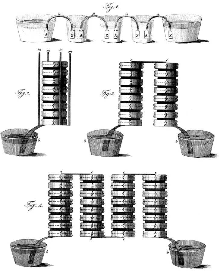
Fire Island runs along the south shore of Long Island, between the ocean and a series of shallow bays. A photograph from May 2009 shows the stretch before the breach. A boardwalk crosses narrow terrain and a sandy ocean beach runs through the frame. Ocean and bay are close to each other here. The place was already known as Old Inlet. A previous connection at the site had been open from 1763 to 1825, carrying fishing and cargo vessels between the Atlantic and the bay. Sand filled in the route, and for nearly two centuries the ocean-facing beach crossed over it. The name outlasted the channel.

An oblique aerial photo from May 2009 shows an unbroken strip of beach. A yellow arrow identifies a small structure on Pelican Island across shallow bay water from a dock.
Before the storm, the beach was continuous here. The yellow arrow in the original points to the fishing shack on Pelican Island that remained standing after Sandy. Cropped from the May 21, 2009 panel of the USGS comparison. · Karen Morgan · U.S. Geological Survey · U.S. public domain · U.S. Geological Survey

Hurricane Sandy opened three breaches in the barrier islands on Long Island’s south shore. Workers filled two of them soon after the storm. The channel at Old Inlet was inside the Otis Pike Fire Island High Dune Wilderness. The immediate response there was to watch it under an existing contingency plan. Amid the far-reaching damage the storm had caused elsewhere, there were practical reasons to track the opening. A new passage could change tides in nearby communities. It could also change the composition of the water and the movement of sand in the bay. Both the depth and the shape of the opening would matter.

A satellite image taken November 3, 2012, gives a first benchmark in the U.S. Geological Survey’s later reconstruction. Gary B. Fisher tabulated a width of 72 metres from that image. By October 2013 a comparable measurement was 190 metres, and a June 2016 image gave 440 metres. Those are measurements at the time the different images were collected, and they describe the width of the open water seen across the inlet. They leave another question for field surveyors. Two channels that look the same width in a photograph can differ in depth, and the submerged cross section helps control how much water can pass.

In the first years, the measurements traced a shifting passage as well as a widening one. The line of the channel marched west, in the direction that sand commonly travels along Fire Island’s ocean shore. Powerful winter storms helped reshape it. Researchers could trace this movement by aligning each image with the same map and drawing the position of the shore at a series of dates. The photos form a sequence in which both banks shift. Simply putting a ruler across one frame captures how wide the channel was at that moment. The sequence shows that an inlet can move while remaining recognizably the same connection.

The current also built a large submerged form in the bay. On the incoming tide, water carried sand through the breach and then spread out, depositing some of it in broad shallows called a flood shoal. The outgoing tide helped form an ebb shoal on the ocean side, which stayed comparatively small. Fisher used images that record several wavelengths of light to delineate the bay-side formation, because the different responses helped pick out the shoal even through murky water. He mapped about 1.04 square kilometres of it in October 2013 and about 2.76 square kilometres in June 2020. Much of this feature lay underwater. Its measured area describes shoal extent, including submerged sand.

The breach also let ocean water reach the eastern bay along a shorter route. The National Park Service and its partners compared tide-gauge records and found that, near the breach, mean high water changed by a small amount relative to the usual range of the tide. In nearby Bellport Bay, high and low tides began to arrive about 20 to 35 minutes earlier in the cycle. The two observations measure different things. One describes how high the water gets on average at high tide. The other describes when the turning point arrives. Opening a channel can change the route a tide takes and show up in its timing even when the routine high-water mark changes little.

The record at Old Inlet offers a local measure of change. A smaller rise in mean high tide near the opening says little by itself about the compound effects of waves, wind and surge spread across Great South Bay during a future storm. That question called for models as well as field records. The Park Service commissioned and reviewed both kinds of work for its management decision, because the shoreline could continue evolving faster than a long record of exceptional storms could accumulate.

Monitoring also detected cooler summers in central and eastern parts of the bay and saltier water after the new connection opened. The Park Service estimated that water in Bellport Bay spent about 40 days there with the breach open, compared with about 96 days before. Such a residence time represents typical circulation, with some parcels leaving quickly and others lingering. It helps explain how the opening could make conditions in the bay different from those a scientist would infer from water levels alone. The agency considered those observations alongside its storm scenarios and its responsibilities for the surrounding communities.

In July 2018 the Park Service approved a management plan that let natural processes reshape or close the inlet while monitoring continued, with provision for intervention to prevent severe harm. By May 2021 Fisher’s image-based width was still 272 metres. The October 20, 2022 image showed just 22 metres of opening. Sand moving along the ocean shore had built out the edge until the passage closed later that year. A December 2023 image shows continuous shore and a bay-side shoal that still measured about 1.29 square kilometres. The water passage had gone, while much of the sediment it delivered remained.

On the first photographs, the two ends look like a broken road waiting to be joined. The decade of mapping shows where that comparison ends. The closing shore formed in a different position, and the beach at the breach site still had a visibly lower profile than it had before Sandy. Inside the bay lay shoals built during the years when the tide crossed there. The old ocean-to-bay passage had closed twice over the historical record, in the nineteenth century and again in 2022. In each case the continuous line on a map hides a coast assembled in a new way.

A clear boot tread impression in gray lunar soil beside undisturbed ground.
A close-up of a bootprint on the Moon during Apollo 11, July 20, 1969. Resized for display. · NASA · Apollo 11 image AS11-40-5878 · NASA media use guidelines

Moon · 6 min read

An Apollo bootprint has no rain to erase it

AI narration · Fraser

There is a photograph from Apollo 11 in which a boot has done almost all of the work. The sole has pressed deep bars into the surface. Along the edge, the material forms a raised lip, and a dusting of finer grains takes the light. The photograph looks ordinary enough to have been made in a garden until you remember where it was taken. On July 20, 1969, during the first crewed landing on the Moon, a lunar surface camera recorded a clear impression in a place with no rainfall and no Earth-like wind to smooth it over.

The material underfoot is called regolith. That word describes the loose material covering solid rock. On the Moon it includes dust, grains, rock fragments and material altered by impacts. Across lunar history, collisions have broken material into smaller pieces and moved it around. On Earth, a handful of soil can contain water, plant material and a living community that changes its texture. The gray material in the Apollo image formed under very different conditions. It can take a visible impression without the rain or dampness you might expect to need from the experience of making prints at home.

Look at the edges in the photograph. The deep grooves and narrow ridges make the tread shape legible, even though the solar light gives some areas more contrast than others. A footprint is a record of displacement. The arriving shape pushes some grains down and some outward. The visible pattern is what remains when the boot lifts away. In a loose material, the fine details that survive depend on what the individual grains do as they are pressed together and released. The picture shows the result for this particular print and surface, without telling you that every part of the Moon behaves the same way.

The difference with Earth becomes clearer if you think of all the things that can change a mark without another person stepping on it. Water drains across bare soil, and later drops strike the ridges. Dry grains can be carried away by air. On a beach, a rising tide can lift and redeposit the sand in a few moments. An impression may look strong just after you make it and still vanish before you return. There are great differences among those places, but most familiar outdoor landscapes have at least one process that gives a fresh footprint a fairly short life.

The Moon has a very sparse exosphere. Scientists study its particles, which include material knocked loose from the surface. Calling it a familiar blanket of air would give the wrong picture. Earth’s atmosphere is dense enough to support the kind of winds that move dust in a field. The lunar exosphere cannot produce the weather you would count on to change the shape of a footprint outdoors here. There are no showers passing through Tranquility Base to smooth the loose material back into place. That absence of everyday weather helps explain why Apollo surface disturbances last so long.

Decades after the landing, the camera aboard NASA’s Lunar Reconnaissance Orbiter looked down at the Apollo 11 site. The image from that mission shows the descent stage, the lower part of the lunar module, and trails left by the astronauts. Think of the scale change between the two photographs. At boot height, you can see bars impressed by the tread. From orbit, you can follow disturbed paths across part of the site. The orbital image does not identify the single close-up impression or reveal its tread pattern. The two pictures answer different questions, and the difference makes the evidence easier to understand.

An overhead orbital view of the Apollo 11 landing site with the descent stage and faint trails across the gray surface.
From lunar orbit, the Apollo 11 descent stage and the astronauts’ trails appear at a scale very different from the close-up bootprint. · NASA / Goddard Space Flight Center / Arizona State University · NASA media use guidelines

A trail can be visible without any one print in it being clear. Many steps close together disturb a longer strip of material, and that makes a larger pattern for a distant camera to distinguish. When you look at the landing site picture, the trails matter because they extend between parts of the scene. The stage is a separate object with a different shape and scale. Read the image as a collection of site features rather than as a magnified version of the astronaut’s photograph. Seen together, the pictures connect a very small moment at the surface with a longer trace of travel.

That persistence does not mean the surface has stopped changing. Small incoming particles strike the Moon, and impacts can scatter fresh material over older surfaces or disturb grains already there. NASA’s studies of the exosphere describe how impacts loft some material. Over long stretches of time, changes of this kind can soften or obscure marks. The photographs tell you that human traces persisted long enough to be observed decades later. They do not supply a reliable expiration date for any given footprint. How long a particular ridge remains recognizable is a narrower question than whether the bigger path can still be seen.

There is a reason to avoid treating the people, the equipment and the prints as three unrelated details. The stage is where the landing machine came to rest. The trails describe some of the activity around it. The close-up records what a boot did at a single spot on the surface. Archaeologists often work with differences of scale like these. A small trace can tell you about contact with a material; a broad pattern tells you how activity was spread out. An image does not have to resolve every detail to answer a useful question about the site.

Next time you see the famous photograph, look first at the places where the tread ends and loose ground begins. On Earth, you can imagine the same print at a dusty road shoulder, in a sandpit or at the edge of the sea. What would reach it before you came back? The answer on the Moon starts with an absence: no everyday wind or rain. The rest of the story is slower and less familiar. Tiny impacts can still rearrange material, but a brief step made during a mission in 1969 was enough to leave a trace an instrument could recognize decades later.

Original dimensional cutaway illustration of a pale fibrous ceramic tile body with a thin dark surface coating on a warm orange background.
Original Atlas explanatory illustration. The body, coating and texture are schematic, not a measured tile or microscope image. · Augustine Atlas

Ceramics · 6 min read

The spacecraft shield that was mostly air

AI narration · Gracie

One of the Space Shuttle’s most important protective materials was astonishingly empty. LI-900, a rigid ceramic insulation used across the orbiters, was made from silica glass fibers with air occupying about 94 percent of its volume. The solid network took up only a small fraction of the space inside an apparently substantial tile. This was not packaging foam tucked somewhere inside the spacecraft. It was part of the system that helped protect the orbiter during its return through the atmosphere, when the outside faced intense heating.

The percentage describes volume, not weight. It does not mean that 94 percent of a tile’s mass was air, or that the tile was a sealed box containing a large bubble. It describes a porous structure: fine solid fibers with a great deal of space between them. That distinction changes the mental picture. A dense block and an airy fiber network can occupy the same external dimensions while containing very different amounts of solid material. An object’s outline tells surprisingly little about what fills it.

The material name is useful because the Shuttle did not have just one universal kind of tile. The NASA Ames materials database identifies LI-900 as an all-silica fibrous insulation with a nominal density of nine pounds per cubic foot, roughly 144 kilograms per cubic meter. Its composition is listed as silicon dioxide, SiO₂. In this context, ceramic does not mean a clay pot or a dense kitchen tile. It includes a carefully engineered high-temperature material whose internal arrangement is essential to its performance.

Published NASA micrograph showing interwoven silica fibers and open spaces, with a nine-micrometer scale bar.
Silica-fiber micrograph from NASA Ames’ 2025 LI-900/LI-2200 presentation, slide 37 (PDF page 35). Cropped to the published image and its 9 µm scale bar; the slide does not identify which of the two grades this specimen represents. · NASA Ames · Reusable Thermal Protection Material Development · NASA NTRS record: public use permitted; no third-party material indicated

The returning orbiter’s problem was not simply that the atmosphere was hot. A vehicle entering at high speed compresses the gas in front of it, creating an extreme heating environment. Thermal protection had to keep that environment from overheating the underlying vehicle. A heat shield therefore involved more than choosing a substance with a high melting point. The material also needed to control the rate at which energy moved inward, survive the flight environment and fit into an aircraft-like structure.

LI-900’s very low thermal conductivity was central to that job. Thermal conductivity describes how readily heat travels through a material; low conductivity slows that transfer. The tile’s sparse fibrous structure provided insulation without the weight of a dense solid block. The important relationship was between its hot exposed side and the structure underneath. It was possible for those regions to be at very different temperatures during heating. The tile was doing useful work precisely because it did not rapidly equalize them.

The familiar dark exterior was another part of the design. Many Shuttle tiles carried a coating called Reaction Cured Glass, or RCG, made with borosilicate glass and a silicon-boride constituent. That coating protected the porous material and provided high emissivity, helping the hot surface radiate energy away. A photograph of a black tile can conceal the fact that its outer coating and pale fibrous body perform different roles. The visible surface is not a complete description of the insulation beneath it.

An excellent insulator can still be mechanically delicate. LI-900 tiles were brittle and vulnerable to impact, and their attachment had to accommodate a vehicle that flexed and changed temperature. Making the underlying aluminum structure carry a fragile ceramic as though the two were one unbroken solid would create problems. Thermal survival, mechanical strength and low mass were separate requirements that sometimes pulled the design in different directions. The tile had to work as part of an assembly, not merely pass a furnace test in isolation.

Between the tile and the orbiter sat a strain isolation pad, commonly abbreviated SIP. This Nomex felt layer helped prevent damaging stresses from being transferred directly into the rigid ceramic. Adhesive bonded the tile to the pad and the assembly to the structure. The pad’s purpose makes the system more understandable: a soft intermediate layer could protect a hard but fragile component. Flexibility in the right place was part of the protection rather than evidence of an insufficiently strong design.

Even that interface required refinement. Concentrated loads associated with the pad’s fiber bundles could damage the ceramic near its attachment. Densifying the tile’s inner surface helped spread the load more evenly and increase strength at the bond line. The result was not one uniform material from outside to inside. It combined an exposed surface treatment, a lightweight insulating body, a strengthened attachment region, adhesives and a compliant pad, with each part addressing a different demand.

Manufacturing brought its own mixture of furnace work and precision shaping. At the Thermal Protection System Facility, tile material is cast into billets and sintered, then machined and coated. The facility uses ovens, mills equipped with dust collection, and specialized staff to make and maintain these components. A finished tile’s geometry is therefore the product of both material processing and careful removal. It belongs to the world of ceramic fabrication, but also to the world of fitted aerospace parts.

Tony Rollins works at a contour milling machine on a white thermal-protection tile at Kennedy Space Center.
Tony Rollins of United Space Alliance shapes an HRSI tile in Kennedy Space Center’s Tile Fabrication Shop, August 10, 1998. NASA image KSC-98pc930; resized and converted to WebP. · NASA · KSC-98pc930 · NASA images and media usage guidelines

Porosity created a less obvious complication on the ground: water. A NASA Ames research report describes how moisture could enter the spaces in silica tiles, increasing their weight and harming their thermal performance. Waterproofing treatments addressed this, but reentry heating removed the treatment, making renewal part of servicing. The same internal space that made the material light had to be managed throughout its working life. A tile’s condition before launch mattered as well as its ability to endure heat during descent.

The rest of the orbiter used other protection where the conditions demanded it. Reinforced carbon-carbon protected the wing leading edges and nose cap. Different reusable tiles and flexible insulation blankets covered other areas. Treating every dark panel or every white surface as LI-900 erases those distinctions. The thermal protection system was a geographic arrangement of materials, matched to different parts of the vehicle, rather than a spacecraft wrapped in one remarkable substance.

Development also continued beyond the original low-density silica tile. Other fibrous ceramics increased strength or durability, and surface treatments improved resistance to damage. NASA’s materials descriptions record FRCI replacing tiles where damage had been an issue, alongside blanket systems and other reusable materials. Better insulation was never the only measure of improvement. A useful successor might trade some mass or conductivity for mechanical resilience, easier servicing or performance in a different heating environment.

The surprising fact survives all these qualifications: an apparently solid protective tile could be mostly empty space. But the fuller story is more interesting than a percentage alone. The empty space belonged to a particular fiber architecture, the architecture needed a suitable surface, and the surface needed an attachment system and maintenance. This is what makes the Shuttle tile a compelling ceramic object. Its achievement came from arranging material carefully, including the places where very little material was present.

Jefferson’s handwritten cipher sheet has a tight grid of alphabet characters, with longer instructions and a sample below.
Jefferson’s April 1803 cipher manuscript. The grid and sample record how he intended to protect a dispatch. Library of Congress scan resized for display. · Library of Congress · Jefferson’s cipher for the Lewis and Clark expedition (exhibit item 55) · Public domain · Library of Congress, Free to Use and Reuse

Cryptography · 6 min read

Thomas Jefferson gave Meriwether Lewis a cipher he never used

Thomas Jefferson put the word artichoke to work in one of the most unusual preparations for the Lewis and Clark expedition. It served as the key in a sample message on a cipher sheet he wrote for Meriwether Lewis in April 1803. The demonstration describes Lewis reporting from the upper Missouri, reassuring Jefferson about the party and its encounters so far. The line of letters and symbols on the original page looks nothing like such a report. It was an example Jefferson wrote at a desk before the journey. The Library of Congress, which holds the cipher, says Lewis never used it during the expedition.

The sheet gives a surprisingly physical answer to a problem of distance. Lewis would have a handwritten chart and a word agreed in advance. Jefferson could have the corresponding information in Washington. If Lewis needed to report on a sensitive matter, he could turn the readable text into a series of characters intelligible to the person who knew how to reverse the transformation. A person who carried the dispatch could keep it moving across the continent without having to know what it said. The president had to design for a route involving people, paper and long pauses between opportunities to send news.

Jefferson's chart was an arrangement of letters, numbers and symbols. In one of the methods described in the earlier version, the keyword determined how the writer used the grid to change a message. This was more flexible than an alphabet printed in a single fixed correspondence. The same letter could take different forms in different positions. That mattered because a simple substitution leaves a recognizable pattern over a long enough text. Here, the sheet and the keyword gave the reader a way back to the ordinary language of the report. The Library of Congress preserves two versions in Jefferson’s hand and identifies the second as the revised one Lewis was given to carry west.

By June 1803, Jefferson had set out the larger assignment in a lengthy letter. Lewis and his party were to follow the Missouri and search for a route across the continent that could serve commerce. Jefferson asked for information on the land and waterways, plants, animals, geology and weather. The letter also asked the party to record the languages, commerce and political arrangements of Indigenous nations. It directed the expedition with the United States’ territorial and commercial ambitions in mind. The nations Lewis and Clark met had their own governments, trading relationships and reasons for deciding how much assistance or access to offer the party.

Jefferson’s instructions reveal what he thought a route for the mail might look like. In the earlier part of the journey, messages could move between settlements and Spanish posts. Farther up the Missouri, traders might be able to carry letters. In places beyond convenient trading routes, he suggested asking Indigenous people to take government dispatches to Cahokia or Kaskaskia in return for an agreed payment. Their geographic knowledge and travel networks, as well as those of traders, could help the expedition communicate. The possibility of those arrangements explains the usefulness of a dispatch the carriers could convey without reading its sensitive contents.

In his June instructions, Jefferson also asked Lewis to make multiple copies of the party’s notes and entrust them to dependable members. He was preparing for the possibility that the records might be lost altogether. A copy carried by someone else could survive the loss of one package of papers. A cipher could protect the sense of a report if it came into another reader’s hands, but the report still had to reach Washington. Jefferson’s plan addressed both kinds of risk on the same page of an actual expedition brief. The handwritten cipher gave Lewis one option for the passages where disclosure could matter most.

A page of the letterpress copy of Jefferson’s instructions to Lewis is closely written in brown ink.
The third page of a letterpress copy of Jefferson’s June 1803 instructions to Lewis. It asks the expedition to record the geography, climate and people encountered along its route. Scan converted for display. · Library of Congress · Thomas Jefferson’s instructions to Meriwether Lewis, June 20, 1803 · Public domain · Eighteenth- and nineteenth-century U.S. presidential papers

When the expedition had an opportunity to send substantial news downriver, its leaders did so in ordinary writing. At Fort Mandan in April 1805, the main party was preparing to travel farther up the Missouri. A separate group took the keelboat downriver toward St. Louis with dispatches and specimens for onward delivery. Lewis’s April 7 letter to Jefferson accompanied an account of what the party had seen and what it was sending. Its surviving text is readable, and the journals record the party’s confidence in the pilot and boat. The documents give us an actual handoff to set beside Jefferson’s hypothetical one. Lewis identified Joseph Gravelines as the pilot, an experienced boatman he trusted with the return journey. Clark’s journal records the two parties leaving the fort in different directions after wintering there. That division let the larger expedition continue collecting information as an earlier set of observations had a chance to travel back toward the president.

That comparison makes the cipher sheet easier to read as evidence. Jefferson’s sample was written in advance. Its upper-Missouri setting and assurance about the travelers tell us what he imagined hearing from Lewis. The Fort Mandan letter was written during the journey and records a different situation, with actual decisions about who would carry the dispatches. Both survive in collections readers can study. Only one was a report sent from the field. The apparent message on the cipher page can look like the missing dispatch if its purpose as a demonstration is overlooked.

We also have little basis to infer from the unused tool that the expedition’s communications posed no risks. Jefferson expected delays. His instructions considered that a party might have to turn back, lose records, or send a copy home by another route. An occasion suited to the cipher would have brought together a sensitive subject, an opportunity to send a letter, and enough time to prepare something Jefferson could read at the other end. The surviving record shows the provision Jefferson made and the dispatches that reached him. It leaves the party’s every private decision out of view.

The curious word at the center of the cipher was ordinary enough to remember, and the handwritten table was compact enough to travel among other papers. That combination tells us how Jefferson imagined secrecy working on this particular expedition. It was a tool one writer would need to use with pen, paper and time, while a second reader would need the right information months or many miles away. Between those two people were boats, settlements, rivers and potential couriers who all had their own part in moving a letter. The expedition left no known dispatch encrypted with this system. The tool itself survives with the communication plan it was built to serve.

Vertical supports surround a tall stack of dark metal discs in a museum display case.
A voltaic pile on display at the Tempio Voltiano in Como. The museum photograph is cropped to show the discs and their supports. · Dario Crespi · Pile at the Tempio Voltiano, Como · Wikimedia Commons · Creative Commons Attribution-ShareAlike 4.0

DC Circuits · 6 min read

Volta’s battery needed wet layers between its metals

On March 20, 1800, Alessandro Volta put the description of a battery into a letter to Joseph Banks, the president of the Royal Society. Its critical feature fit into a repeating stack. Pairs of metal discs sat one above another, with wet pieces of porous material separating successive pairs. Keep the metals in order and add more repetitions, Volta reported, and the effect grows. The wet layers were as essential to this source of electricity as the gleaming metal. For a researcher accustomed to static charges and short discharges, the stack offered something different. It could keep current moving through a closed circuit.

A pile displayed in the Tempio Voltiano in Como gives that description a shape. Narrow vertical supports stand around a column of tightly packed discs. Seen at a distance, it resembles a single dark cylinder. Up close, the edges reveal how many separate pieces are present. The supports help the layered stack stay upright and aligned. The photographed object is a museum example of the apparatus. The arrangement Volta circulated in 1800 survives separately, in his letter and in the illustrations printed with its published version.

Volta described several materials that could be used. He preferred silver or copper paired with zinc, and he could use porous material such as cardboard or leather for a separator. A conducting liquid, such as salt water, went into the porous layer. The structure depended on repeating the order, a detail with electrical consequences. If each unit contributed a small electrical potential difference with the same orientation, its contribution would add to those of the other units. In modern terms, the repeated cells in the pile were connected in series. The voltage between the two ends could be appreciably larger than the voltage from one cell.

The wet separator lets ions move. Ions are atoms or groups of atoms carrying electric charge. In the pile's metal parts and its external wires, electrons carry the current. A battery can couple these two forms of charge motion through reactions at the surfaces where metal meets the conducting liquid. Zinc can enter the solution as positively charged ions, leaving electrons behind in the metal. At the other electrode, reactions take up electrons. The exact chemistry depends on the metals and liquid. The external path and the path through the liquid both matter to a circuit that can keep operating.

Volta's own account and the modern electrochemical account assign different roles to the materials. He attributed the electrical force chiefly to contact between unlike conductors and called attention to the effect of keeping them in a consistent order. Today the sustained delivery of energy is understood through the chemical reactions and the movement of charge in the whole cell. The stack could work, and people could reproduce it, while its explanation was still a question for experiment. That distinction matters when reading the original paper. It reports a working design even where its author's interpretation belongs to an older account of electricity.

The published plate documents a second shape for the same basic idea. Across the top, small cups form a line, with curved metal connections between neighbors. The cup form separates the liquid into containers and makes the repeating links easy to see. Underneath, the drawings show a tall column and then arrangements of multiple columns. The artist could expand the number of units across the width of the page while keeping their relationship visible. Volta's proposal was a way of combining repeatable elements. It could take the form of a long row of cups or a compact stack of discs.

An engraved plate shows a row of linked cups at the top, a single narrow column and two paired columns in the middle, and four columns at the bottom.
Plate VIII from the 1800 publication. The top figure shows the linked cups. Below are examples of the column arrangement. Resized for display. · Alessandro Volta · Plate VIII, Philosophical Transactions, 1800 · Scan via Wikimedia Commons · Public domain

One familiar instrument helps explain the novelty. A charged Leyden jar stores separated electric charge. Connect a path across it and it can discharge rapidly, giving a noticeable shock or spark. To repeat the discharge, an operator must charge it again. The pile used chemical energy and could maintain a potential difference as current flowed. Researchers could observe electrical effects over a longer interval as well as repeating them. The distinction concerns what happens after the circuit is closed, especially the time course of the current. A dramatic spark alone says little about how long a source can continue to power a process.

The supply from a pile was imperfect. Adding layers could increase the potential difference, but the stack and all its wet separators also contributed electrical resistance. Liquid squeezed from the separators could run down the outside and allow current to bypass part of the stack. Gas could gather at an electrode and interfere with the cell’s delivery of voltage under load. The cups gave the conducting liquid separate containers, reducing the risk of a spill linking several cells accidentally. A tall stack also had to keep many soft and hard layers in contact and in order. The uprights visible on a museum pile tell part of the engineering story that a simple circuit symbol leaves out.

The Smithsonian's National Museum of American History catalogs an example dated 1805. Its record identifies a pile using zinc and copper discs with cloth soaked in salt water between the pairs. That example helps show how the design traveled beyond the exact material choices Volta described. Silver might appear in a description, and copper could appear in an actual instrument. The repeatable element was a set of conditions that had to be met. The pairs of metals had to be arranged in the appropriate order, and the wet layers had to permit charge to move within the cells.

Continuously available current changed what could be investigated. A brief electrical discharge is over in an instant. A current maintained in a circuit gives an observer time to see the products of a chemical change accumulate or to compare the effect of inserting different materials into the same path. Other battery designs later improved on the pile. The initial advance was already visible in the 1800 drawings, where the arrangement of many little units is drawn carefully enough to show how they belong to one instrument.

Modern battery packs still reveal the value of keeping the sequence straight. A holder can join two identical cells so the voltage at its outer terminals is approximately the sum of the individual cell voltages. The case and metal contacts hide most of what goes on inside a cell. Volta's arrangement puts the repeated parts in plain view. The person looking at the apparatus can count many of the layers and see the materials that made a continuing current possible. A small stack of parts changed the kind of electricity available on the laboratory table, from something researchers could briefly release to something they could use while a process unfolded.

A cropped 1693 print of Halley’s opening title sits against dark green next to the figures 445 and 377.
Opening of Edmond Halley’s 1693 paper, p. 596. Atlas cropped and tinted the scan and set Halley’s later example beside it. His table listed 445 people at age 40 and 377 at age 47. · Edmond Halley · Philosophical Transactions 17 (1693), pp. 596–610 · Royal Society via JSTOR · Public domain · Creative Commons Public Domain Mark 1.0

Demography · 6 min read

Edmond Halley used a city’s burial records to put odds on seven more years of life

On two pages of a paper published in 1693, Edmond Halley posed a compact question. What odds did a 40-year-old man have of living seven more years? Halley turned to a printed table. In its columns there were 445 people at age 40 and 377 at age 47. The difference was 68. He put the odds in favor of survival at 377 to 68, about five and a half to one. This was a way to give a numerical answer about the future using five years of records from Breslau, the city now called Wrocław, Poland.

The records came from a source that did business in whole events. The town’s bills of mortality, as Halley described them, recorded births and supplied monthly information on burials, including ages and sexes of the people who died. Halley said that a correspondent identified as Mr. Justell had communicated the tables to the Royal Society. The figures covered 1687 through 1691. They told him how many deaths occurred at different ages in those years. They gave him a shorter view than the lifetime of any of the adults whose chances he wanted to calculate.
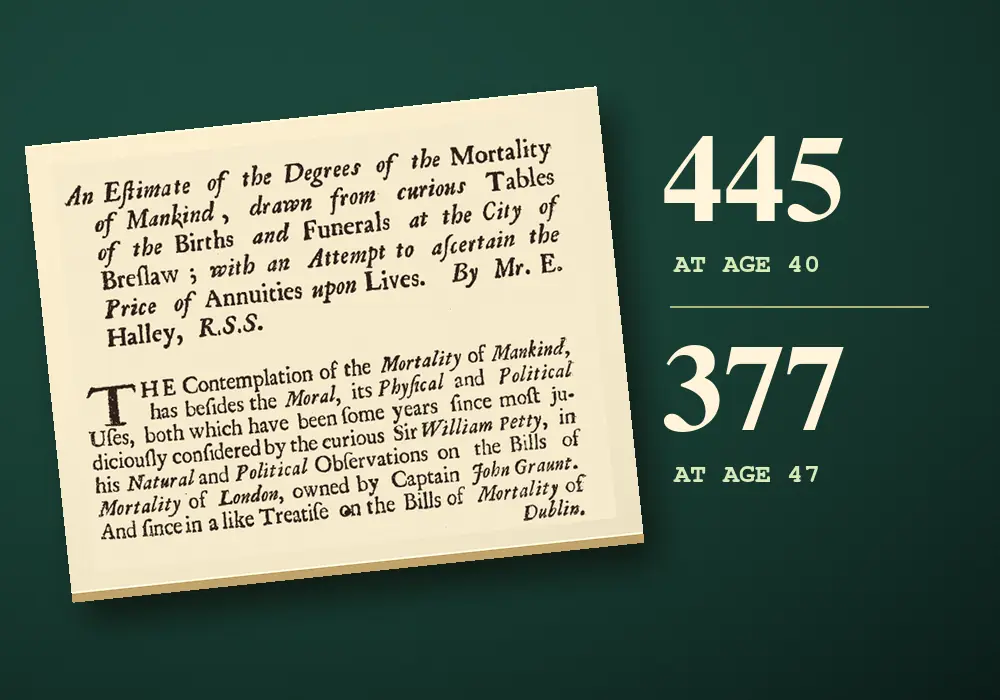
Halley began with 6,193 births and 5,869 burials across the five years. He stated the annual averages as 1,238 births and 1,174 burials. Those totals gave him an idea of the scale of the city’s recorded vital events. They also showed the problem with drawing a conclusion from a death count alone. Suppose there were a dozen deaths in a given age band. A dozen out of a few dozen people alive at that age would imply a much higher chance of dying than a dozen out of several hundred. To estimate the odds Halley needed a figure for the people alive and exposed to that risk.
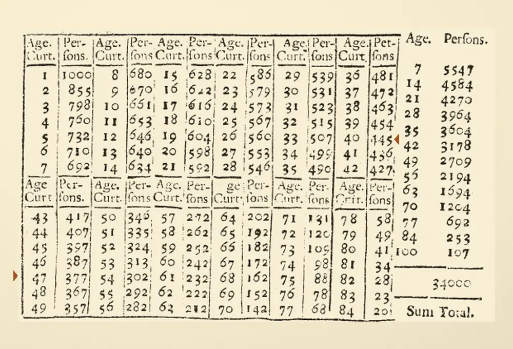

A major assumption concerned movement. In his opening discussion Halley pointed to London and Dublin, where arrivals and departures could complicate the connection between local births and burials. A person could appear in the city’s burial counts decades after being born elsewhere. Conversely someone born in the city could move away and die outside its records. Halley thought Breslau’s inland location and economy made it a more suitable case and considered whether military recruitment could offset the small excess of births he found. His text leaves these as judgments about how much the city might be changing.

Within the five years Halley could compare deaths at many ages. The span of adult life in his printed table came from putting those age patterns together. In the text before the table he reported an annual average of about 348 deaths among babies under one year of age and about 198 across the next five years of age. He also noticed ragged patterns in the teenage years. Some ages had conspicuously few deaths. Halley said a longer record, perhaps twenty years, might smooth out that variation. One thin spot in the record could otherwise turn into a deceptively sharp change along the age sequence.
Two stacked blocks of tiny printed age-and-person columns. Two orange markers in the margins point to the rows containing ages 40 and 47.
Halley’s published survivor table, p. 600. Look for 40 and 445 in the far-right age-and-person pair of the upper block, then 47 and 377 in the far-left pair of the lower block. Cropped and enlarged. Atlas added the orange margin markers. · Edmond Halley · Philosophical Transactions 17 (1693), pp. 596–610 · Royal Society via JSTOR · Public domain · Creative Commons Public Domain Mark 1.0

Look at the printed grid and the design of the evidence becomes visible. The age and persons columns are repeated across the page, so ages advance down a pair and then carry on in the next pair. Halley also distinguished the early death counts in the text from the constructed figures in the final table. The grid supplied the estimated number alive at each age. To get from one age to another you began with the people at the first age and asked how many remained at the second. The family histories behind individual burial entries were outside that calculation.

His answer for seven years can also be expressed as a probability. Of the table’s 445 people at age 40, the 377 at age 47 are the implied survivors, so the probability is 377 divided by 445, about 85 percent. The odds Halley used divide the survivors by those who would die over the interval, giving 377 to 68. The distinction matters because the probability and the odds have different denominators. The two expressions describe the same model and apply only after the starting condition, reaching age 40, is met.

Halley asked a different question for a person aged 30. At what later age would survival be about an even wager? His table gave 531 people at age 30. He halved that number and looked down the list for roughly 265 survivors. The corresponding age fell between 57 and 58. In modern terms, that is a median implied remaining lifetime of around 27 to 28 years conditional on reaching 30. An average would be a different calculation, since it would depend on the length of all the remaining lives represented by the table, including the longest ones.

One of Halley’s applications occupied several pages. A life annuity could pay a sum each year while the person named in the agreement remained alive. A payment expected next year and a payment expected decades later had two different sources of uncertainty or discount. The recipient had to live long enough to receive the later payment, and the present equivalent of money paid far into the future could be smaller. Halley used the survival table for the first part and a specified interest assumption for the second. He then summed the estimated present values associated with payments at successive years.
This was a particular historical calculation based on a particular set of burial records. An outbreak within those five years could influence the death counts. The custom for recording a death or assigning an age could influence them too. Halley needed an approximate link between the annual pattern by age and the structure of the population. If the number of births had been changing rapidly, or if many people of one age had just moved to the city, there could be an age pattern in the data that a survival calculation alone could not explain.

The comparison of 445 with 377 looks as though the same names could be followed from one row to the next. Its arithmetic rests on the particular kind of comparison the table made possible. Halley used the city’s recent record across many ages to construct a set of ages through which a person could hypothetically pass. To an individual 40-year-old, the future still included changes in work, disease and circumstance that had yet to occur. The printed table made visible both what he could compute and the distance between recorded events and a future life.

A juvenile planthopper with a dark banded abdomen and small legs rests on pink human skin.
An Issus coleoptratus nymph photographed at Arnhem in the Netherlands. Skin texture helps convey the small size of the animal. Cropped and resized for display. · Bj.schoenmakers · Wikimedia Commons · CC0 1.0

Entomology · 6 min read

A young planthopper has working gears in its hind legs

In a high-speed recording of a young planthopper, two tiny rows of teeth meet beneath the insect. One row turns and catches a tooth on the other side. Then both hind legs swing into a jump. The teeth are part of the insect’s outer skeleton. In 2013, zoologist Malcolm Burrows and biomechanist Gregory Sutton showed that the teeth in young Issus coleoptratus engage in sequence, coupling the motion of two moving parts just as the teeth on a pair of gears do.

The jobs of powering a leap and timing it are easy to confuse. A planthopper’s large thoracic muscles provide the power. The insect can store energy before the jump and release it rapidly. Timing is a separate problem. If the two legs drive against a perch together, they can launch the insect without a large sideways twist. If a strong push comes from one side first, the body can turn before the other side catches up. That unwanted turn is yaw, the kind of rotation you would see if you looked down at the insect from above.

Imagine pushing a lightweight tray across a table with a finger at either end of its near edge. Give both ends a simultaneous shove and the tray can go straight. Give one end a head start and its far edge starts to turn. The planthopper’s legs are rotating joints pushing against an irregular perch, so the tray is a simplified picture. The useful comparison is the delay. When the entire push lasts around two milliseconds, even a small delay can occupy a meaningful fraction of the launch.

The researchers measured the beginning of the two hind legs’ propulsive movement within 30 microseconds of each other in their recordings of free jumps. One microsecond is one millionth of a second. The nymphs in those trials could accelerate to takeoff in about two milliseconds. If you stretched a two-millisecond push out to two full seconds, the same timing gap would stretch to 30 milliseconds. Consider how closely two moving joints have to agree when each already has muscles working on its own side.

The gears sit on the inward-facing sides of the hind trochanters, leg segments near the body. Each toothed strip in the specimens measured roughly 350 to 400 micrometers, less than half a millimeter. The strips carried ten to twelve teeth, with matching counts on the two sides of a nymph. Their one-to-one ratio couples the speed of rotation. As the joints turn in opposite directions, one tooth steps into the space between its partners and the next takes its turn. A row of teeth along part of each joint is enough for the range of motion used in the leap.

This particular match appears only on the pair of legs that power the jump. The front and middle pairs carry on their own work without these teeth. In photographs of the dissected hind-leg joints, the toothed surfaces face inward toward the body’s center line. The geometry puts the contact where it can join the motions of the two legs without either one having to cross the other’s path. In the drawing, the opposing arcs turn in opposite directions and the teeth travel in the same direction where they touch.

An orange toothed arc on the left meshes with a yellow toothed arc on the right. Arrows by the two pivots show opposite rotations.
Original schematic of the opposing toothed surfaces. The two hind trochanters rotate in opposite directions. The gear shapes and proportions are simplified. · Augustine Atlas · Based on Burrows and Sutton (2013), fig. 1

Under magnification, the teeth have uneven profiles and a rounded transition where each one meets the strip. The researchers compared that rounded base to the fillet used to reduce stress at the base of a manufactured gear tooth. The profiles in the insect are asymmetric, consistent with the fact that the forceful part of the action drives one way. The joints also move back to get into position for the next leap, and the teeth engage during preparation as well as at launch. The two phases put very different loads on the structure.

A close view of the teeth suggested a mechanism, but the researchers needed to show that engagement mattered during motion. Their high-speed recordings let them follow the position of individual teeth. Sometimes the first few teeth slipped past without catching. For a moment one leg was ahead. When a tooth finally contacted its partner, the delayed leg began to move rapidly. The camera had caught a case in which the timing changed with contact. The matching shapes had a measurable consequence.

A second experiment used the insect’s anatomy as a mechanical test. With the legs cocked in the jumping position, the researchers manipulated the tendon of a large jumping muscle on one side. The opposite leg moved promptly, even in a dead specimen. A neural command could not explain that response. The two joints were physically connected through their teeth. In a living jump the nervous system still coordinates muscle activity, and both sides contribute force. The linkage helps account for the tighter match seen at the joints.

The authors watched the mechanism at different scales. They recorded free jumps to capture the way the body and legs moved together. For a clearer view of the small joints, they positioned a nymph on its back with its legs free and recorded the gears themselves. That view makes the moment of engagement observable at a scale that a wide recording of an entire leap cannot offer. The two views connect the intricate movement beneath the insect to the trajectory a person can see.

An adult of the same species takes off with the gear teeth gone. They are lost in the final molt, and the adult continues to synchronize its hind legs through frictional contact at their bases. In earlier performance trials, Burrows recorded a particularly fast male reaching about 5.5 meters per second in under a millisecond. The disappearance of the teeth therefore does not mark the disappearance of powerful jumping. It shows what a different arrangement of the leg bases can accomplish as the insect develops.

Why the adults use this arrangement remains an open question. The researchers suggested that a nymph could replace a damaged gear tooth at the next molt, whereas an adult has already reached its final outer skeleton. They also raised the possibility that the larger adult structures make frictional coupling more effective. Both ideas describe plausible advantages. Comparing the two stages establishes that the coupling changes, and measurements of the jumps establish that both systems work. Those observations leave room for more than one explanation of how the difference arose.

The lead photograph gives the scale of a whole nymph. Looking at it from above, you can see why the small contact surfaces at the inward sides of the hind legs require a different view. The evidence in this study came from bringing those surfaces into view and then catching a change in what the legs did when a tooth engaged. A jump that seems instantaneous contains a brief sequence of events. At the moment one tooth catches, a second leg swings, and a launch less than a blink long stays on course.

An installer stands beside gray lap siding and yellow drainage material exposed above it around a white-framed window.
Drainage material is visible above the siding before the wall is closed. This is a construction photograph of one drainage approach. Converted for display. · Buildprodinfo · Rainscreen.jpg, Wikimedia Commons · CC BY-SA 3.0

Building Envelopes · 6 min read

A wall can stop dripping and still hold water

A vertical sheet of clear acrylic looks like an easy thing to drain. Spray it with water while it stands on end and the rivulets converge, gather speed and fall from the lower edge. Then the dripping stops. A glance at the wall of a shower tells you there can still be water on a surface after this moment. In 2009, building scientists John Straube and Jonathan Smegal reported how much remained in a series of drainage experiments. A single vertical acrylic sheet held about 65 grams per square meter after drainage. Two acrylic sheets separated by a one-millimeter gap held 23 and 25 grams per square meter in two separate tests. An extra surface and a small space between the sheets had produced less short-term storage in that particular setup. Spread over a square meter, the 65 grams represent roughly four tablespoons of water.

Most of their experiments were aimed at a hidden part of a wall. The visible covering, or cladding, can intercept much of the rain driven against a building. Some water can slip behind it through joints or other openings. A drained assembly has room for that water to run down and a way for it to reach the exterior. The hidden surface that receives and routes it is commonly described as a drainage plane. In a working assembly, the surface, the drainage space and the outlet do different jobs. Rain can run off freely on the face while a smaller amount follows a separate path behind it.

The researchers built a balance to find out how much remained behind the cladding after an injection of water. Wall specimens can weigh hundreds of kilograms. The suspension system used a load cell to detect a mass change of a few grams, and calibration weights helped check the response before testing. A separate measurement could capture the mass that drained from the specimen. The two sides of this accounting mattered. A collection vessel below the wall measures what escaped. A change in the weight of the wall reveals how much was still there when the visible flow had slowed or stopped.

For a typical larger specimen, the team introduced water in two portions of 1.5 liters. They used smaller portions for smaller panels. In these trials visible drainage ended about one to two minutes after the team stopped adding water. The researchers could then inspect a short-term retention figure while keeping the exposure brief. A longer spell of wetting would give absorbent materials more time to take up water. The test focused on the mass water still added to the assembly after a short dose and rapid drainage.
The simple acrylic trials were a way to take porous material out of that question. Acrylic hardly takes up water in the way an unfinished wood board does. Yet the exposed sheet still retained beads and patches of surface water. The team also tested hanging polyethylene. Three spray trials on that surface averaged 35 grams per square meter, compared with roughly 65 for the acrylic. Two surfaces can look similarly smooth and still hold different quantities of water. The researchers suggested that the surfaces’ different affinities for water could help explain the result. That interpretation concerns the way water sits on the surface at the end of drainage.

The acrylic pair made the comparison stranger. Washers held the approximately one-millimeter space between the stiff sheets. After each of the two tests the researchers found less water in the space, per square meter of tested area, than the single sheet had held. They suspected the space might have limited the ability of large beads to form. The experiment measured mass, so the proposed explanation remained a hypothesis about the droplets. The comparison also combined different arrangements. One result came from spraying a single surface and the other from testing a drainage gap between two surfaces. The numbers describe those setups and the stated test methods.

Horizontal scale showing 23 and 25 grams per square meter for the narrow acrylic gap tests, and about 65 for a single vertical acrylic sheet.
Atlas redraw of measurements reported by Straube and Smegal, 2009. The gap values are two separate runs. The acrylic arrangements used different test methods. · Augustine Atlas

The more varied wall specimens gave a complementary result. Across the tested assemblies, the authors found no clear correlation between width and short-term retained mass. The materials lining the gap, the shapes of siding components and the actual path water could take all mattered. Untreated cedar held the most water among the tested lap sidings. Nonabsorptive vinyl came next in that comparison. The authors pointed out that the shape of its extruded profile created channels where water could collect. A wall detail can store water by giving it a pocket, even when the material itself absorbs very little.

They used dye to see where water was going behind some of the lap siding. Much of it escaped after crossing only a couple of courses and continued down the outside face. This is one reason a drainage path is easier to understand when a drawing shows the actual profile of the siding. A neat vertical arrow behind an entire facade suggests one continuous journey toward the bottom. Overlapping boards can create shorter journeys that return water to the exterior at several levels. Both observations can fit inside the same broad idea of a drained cladding.

A narrow continuous gap could convey the water delivered under the test conditions, even in one assembly with a barely measurable gap. That result answers a flow question for the tested specimens. A wall in service has additional demands. Its drainage route has to stay open through junctions and construction tolerances. Contact between moving water and neighboring layers can change with the geometry. Air exchange in a cavity can also assist drying of the water that gravity leaves behind. The researchers discussed this work separately from their investigation of gap drainage. Moving liquid down quickly and removing the remainder from damp surfaces take place on different timescales.

The distinction between water that leaves and water that stays matters when the weather comes in episodes. Imagine two bursts of rain a few hours apart. Both could produce an impressive stream from a wall’s drainage outlet. If some of the first dose is still on surfaces or in the material when the second arrives, the next wetting event starts with a different wall moisture condition. A drainage test can quantify short-term storage. Observations over a longer period can show how the same layers dry between storms. Keeping those measurements separate helps explain why the researchers bothered to weigh a wall after the last drop had fallen.

An opened red coffee cherry rests on fingers, revealing two pale seeds.
Two seeds inside an Arabica coffee cherry. During washed processing the skin and pulp are removed, and a slippery layer called mucilage can remain around the seeds. Resized for display. · Roger Burger · Open coffee cherry, Wikimedia Commons · CC0 1.0 Universal

Lactic Fermentation · 6 min read

Time in a fermentation tank can change how coffee tastes

At a coffee farm in Yunnan, China, researchers split freshly harvested Arabica cherries into batches. As part of the experiment, some of the coffee seeds spent longer underwater while they fermented. After every batch had been processed, dried, roasted and brewed, a tasting panel detected a difference. Across the treatments in that trial, the coffees from the longer fermentations had more prominent fruity notes and higher perceived acidity. The cherries had come from the same cultivar, Catimor. Repeating the processing trial a week later helped the researchers assess the effect of the individual steps.

The object that went into the tank was far from the brown bean that goes into a grinder. A coffee cherry is a fruit, typically with two seeds inside. Beneath its skin and flesh lies a slippery, carbohydrate-rich material called mucilage. It surrounds the parchment layer that encloses each seed. Pull away the flesh and some of that coating can cling to the seed package. One job of washed processing is to remove it. The material is familiar to growers because its slipperiness changes how the beans feel when they are handled.

Wet processing gives that coating a place to go. A depulper takes off the skin and most of the flesh. When the resulting seeds are held underwater, soluble material from the mucilage can move into the surrounding water and become available to microorganisms. The researchers found an active community of lactic acid bacteria in their Yunnan tanks, particularly members of Leuconostoc and Lactococcus. They also detected yeasts and other bacteria. The term fermentation here describes activity in the tank, where sugars from the fruit enter a changing chemical environment. The processed beans will still go through washing, drying and roasting before they are used for a drink.

A row of open rectangular coffee fermentation bins stands beneath a roof, with a green rail along one side.
Coffee fermentation bins. The photograph shows the kind of equipment used during wet processing. Zhang and colleagues ran their comparison in concrete tanks in Yunnan. Resized for display. · Ronchy~commonswiki (attributed) · Coffee Fermentation Bins, Wikimedia Commons · Public domain · Rights holder’s dedication

The researchers used two methods to prepare beans for the tank. One was conventional depulping. The other used machinery to strip off the mucilage before the beans entered the water. They tested shorter and longer fermentation times with both methods. For the normally depulped coffee, the standard interval lasted until workers judged that the mucilage had come off. It was 36 hours in the first trial and 48 in the second. The comparison beans that remained submerged from those same batches spent 84 hours in the tank. Working from a split batch gave the team seeds with shared starting conditions, so the extra time could be compared with time spent under otherwise similar processing.

An additional branch tested an operation that looks deceptively similar to fermentation from the outside. After washing, some of the beans were transferred to clean water for a day of soaking before drying. Other washed beans went straight to drying. The water in the second operation had a different starting composition. When the team compared what was in the beans before and after that soak, it found that soaking could reduce some chemical differences that had developed in fermentation. The tasting results therefore belong to a sequence of operations. A step later in the chain can alter the traces left by an earlier one.

The team sampled the waters and the beans along the way. The two locations offered different clues. The water carried sugars and other material from the fruit and acquired compounds from microbial activity. The beans had their own chemistry. They are seeds that remain metabolically active during processing. They respond to changing conditions, including the low oxygen they encounter under water. A molecule found in the tank and in the seed can reflect several routes by which material changed or moved. Measuring both is a way of following the process without assuming that every compound in the seed came from the surrounding liquid.

The researchers carried the comparison all the way to a tasting panel. A cup is separated from the wet tank by drying, the removal of parchment, roasting and brewing. That distance makes the result more interesting. In the study’s analysis, fermentation duration affected more of the measured sensory attributes than either the mechanical removal of mucilage or the added soak. The panel’s average ratings remained fairly close across the samples. Even so, longer fermentations were associated with higher ratings for fruity aroma and flavor and for perceived acidity. Some other notes, including cereal aroma, tended to rate lower with longer fermentation.

The team also measured volatile compounds in the brewed coffee. These are molecules that can move from the liquid into the air and reach the nose. Several compounds with different reported aromas changed with the processing. A fruity rating by a person integrates the mixture they smell and taste, so the result describes the cup as a whole. Testing both the volatile compounds and the panel’s ratings gives researchers separate ways to ask how a change in processing made it to the drink.

A previous field experiment with Arabica of the Typica cultivar in Ecuador had also found differences in cup profiles after longer fermentation. The two studies used different locations and varieties, so the resemblance is interesting even though the tanks and conditions were different. Both experiments give concrete evidence that changing the handling of coffee fruit before drying can be detectable in a finished cup. Each farm works with its own mix of temperatures, fruit, microbes and available equipment. The numbers from Yunnan describe the trial conditions. A processing time on its own leaves those other variables unresolved.

The results also make it easier to understand a word you might see on a bag of coffee. “Washed” can identify a family of processing choices. It tells you something about how the fruit and coating were dealt with, while leaving room for different machinery, fermentation times and soaking decisions. Two bags can both say washed, even if one comes from seeds whose mucilage was largely removed by machine and another comes from seeds that stayed in a fermentation tank while the coating loosened. The word gives you one part of the handling history. A grower’s description of the individual steps gives you more.

Fruitiness in this experiment was a rating of the brewed coffee. The researchers compared groups under shared tasting conditions. They also examined compounds and microorganisms during the wet processing itself. Those are complementary kinds of evidence. The panel tells us that a difference reached the cup. The tank samples tell us that the bacteria, the surrounding water and the seed chemistry were all changing along the way. Together they locate some of the work behind the flavor in a place most coffee drinkers never see, while the coffee is still a living seed surrounded by the remains of a fruit.

A tapering wooden lattice tower rises high above trees and low vegetation, with an observation platform at its top.
The 1890 tower at Station Green in Jennings County, Indiana. The survey report puts the instrument 46.3 meters, about 152 feet, above ground. Archival photograph converted for display. · NOAA Historical Collection · U.S. Coast and Geodetic Survey photograph · Public domain · NOAA federal material

Geodesy · 6 min read

Surveyors used a 152-foot tower to measure angles in Indiana

The wooden scaffolding in the 1890 photograph rises above the trees in a series of narrowing stages. The point the surveyors cared about was near the top. The U.S. Coast and Geodetic Survey’s published account puts the measuring instrument at Station Green 46.3 meters above the ground, about 152 feet. That height bought a clear line of sight to other survey stations. Similar observations, linked together over many years, created the first transcontinental arc of triangulation in the United States.

Look at the tower with an angle in mind. An angle at a survey station is the turn from a sight line to one distant target to a sight line to another. A theodolite, an instrument with a telescope and graduated circles, measures that turn. A ridge or stand of trees can take one target out of sight. From the ground, the observer might have a fine view in one direction and still be unable to make the measurement. The added height made it possible to see across obstacles and to include a particular pair of stations in the same set of observations.

A well-measured baseline gave a group of triangles its scale. Suppose surveyors choose two stations with a clear 1,000-meter baseline between them. At each end they sight the same distant target and measure the angle between their baseline and the target. On a flat diagram, draw the two sight lines from the ends. They meet at the target’s position. With a 45-degree angle at both ends, the target lies 500 meters perpendicular to the midpoint of the baseline. No one has to carry a chain directly from the baseline to that target to establish where it is. This small example uses plane geometry. Long lines across a continent require calculations that account for Earth’s curved reference surface.

Once the lengths of the other sides are determined, one of them can furnish a side for the next triangle. Additional lines provide ways to check the geometry. A network can include multiple routes to the same point and a newly measured baseline to compare with the lengths carried forward by angles. Good triangles matter because a small shift in a sight line changes the estimated point of intersection. If the two lines meet at a very shallow angle, that intersection can move a long way from a small reading error. Sites and triangle shapes had consequences for the quality of the final result.

The 1900 report lists the Indiana tower as scaffolding at Station Green. NOAA’s later photo caption spells the station name Greene. In the survey’s calculations a side between Green and Stout comes out to about 28.43 kilometers. The account traces the length back to the measured Holton base. That pairing makes the photograph more specific. A tall tower above the treetops could look like a lookout. Its published purpose was to furnish observations that could establish relationships among named points separated by tens of kilometers.

The work extended from 1871 into the late nineteenth century. In the western sections, mountain summits could give crews the height they needed, while those same sites raised problems of weather, access and altitude. In wooded or flatter stretches, crews sometimes had to construct the height themselves. NOAA’s history says the tallest tower associated with the arc reached 275 feet. The 39th parallel gave the project an east–west corridor to follow. The stations could depart from that latitude so that they could see one another and form useful triangles.

Getting high enough was only part of getting a usable view. At a distant station, a surveyor could aim a mirror toward the observing telescope and make reflected sunlight serve as a target. The mirror instrument was called a heliotrope. A photograph in the 1900 report shows the observation setup on Colorado’s Uncompahgre Peak for a sight to a heliotrope on Utah’s Mount Ellen, a line the report gives as 294.1 kilometers. Imagine finding a point of reflected sunlight on that far part of the horizon. Both ends of the observation needed preparation.

An archival map of the contiguous United States with interconnected triangles extending from coast to coast.
The U.S. Coast and Geodetic Survey’s 39th Parallel Arc. The network ran generally east to west, using observable stations away from the exact latitude where needed. Image resized for display. · U.S. Coast and Geodetic Survey · Map of the 39th Parallel Arc, NOAA Central Library image theb1569 · Public domain · NOAA federal material

The archival map makes that choice visible. Look at the lines as relationships between stations. They cross empty-looking places on the printed page because the observations connected selected points, not because someone traced one continuous route at ground level. The surveyors had to reach the stations, bring or build what they needed, put up targets, and get conditions that let them see each other. The readers of the finished report could then trace how the observations connected. That ability to audit relationships was one of the network’s accomplishments.

The geodetic problem also reached beyond getting from one coast to another. Suppose neighboring regions each surveyed their own towns and roads to a high local standard. Where their surveys meet, the points may disagree if the regions chose different starting coordinates or orientations. A common network provides points that both groups can use. The transcontinental arc, together with connections to independent surveys on the West and Gulf coasts, contributed to a readjustment and the official United States Standard Datum of 1901. The sites on the map helped determine a common coordinate system that later surveys could work from.

Schott’s published volume also uses the long arc as input to questions about the Earth’s figure, the shape and size represented by the geodetic model. A continent-wide comparison forces small assumptions to add up over a substantial distance. A local triangle might look convincingly flat even though projecting that approach across thousands of kilometers would fail. Measuring across a wide span and comparing geodetic results with astronomical observations gave the survey another way to assess the reference model. The angle observed at a tower had a place in a much bigger calculation than the two targets framing it.

Consider how much of this work the photograph conceals. The wood and platforms got the observer above the obstacles, but the instrument still had to be positioned and the sights taken carefully. Other crews had to establish targets and tie their own observations back to the same stations. Workers later had to decide how to reconcile measurements that did not agree perfectly. The monument at ground level, the instrument above it and the line in the report each preserve a different part of that work.

Modern satellite positioning can connect many stations that cannot see each other directly. That change makes the tower look like an answer to a remarkably specific problem. It gave people working with a telescope an unobstructed view of the selected target. Once that one direction was observable, it could be compared with another, combined with readings from other stations, checked against measured lengths and used again. The height of the scaffolding was dictated by what the landscape hid. The resulting observation could travel much farther than the view from the top.

An oblique aerial photograph shows white Hubbard Glacier pushing a dark ridge of sediment against the green shore at Gilbert Point.
Hubbard Glacier’s 2002 closure on July 16. The gray sediment ridge meets the opposite shore between the white glacier and the green slope. Converted for display. · U.S. Geological Survey · July 16, 2002 photograph, via Wikimedia Commons · U.S. public domain · U.S. Geological Survey

Glaciology · 6 min read

An advancing glacier turned an Alaskan fjord into a lake twice

In July 2002, a photograph taken above the entrance to Russell Fiord showed white, fractured glacier ice coming down to the water in southeastern Alaska. Between the ice and a green hillside lay a dark ridge of sediment. On one side of the ridge was Disenchantment Bay, connected to the Pacific through Yakutat Bay. On the other was a basin that could no longer rise and fall with the tides. Hubbard Glacier had pushed sediment against the shore and turned a roughly 60-kilometre-long fjord into a lake.

A fjord can have a narrow opening even when it stretches far inland. Near Gilbert Point, there was a relatively short gap between the shore and one part of the wide glacier front. As long as the gap stayed open, tides could drive water through it in both directions. Rain, streams and glacial meltwater also supplied the basin. An incoming tide might briefly raise water in both the bay and the fjord. Over longer periods the open passage gave the freshwater an outlet. Blocking the gap changed the budget for the entire inlet.

Hubbard is a tidewater glacier, meaning part of its edge ends in seawater. When chunks break away from that edge, they become icebergs. Ice flows in from farther up the glacier and can replace what breaks off. The front’s position also depends on what lies beneath it. A shallow bank can help keep the ice grounded and affect how quickly the front loses ice. As Hubbard advanced, it pushed up sediments that had been lying under water near its leading edge.

In spring 2002, the sediment ridge emerged above the water surface. An aerial photograph from May 20 showed the sediments building up while tides still moved through the opening. By mid-June a ridge had reached the rock wall, and tidal exchange stopped as the connection closed. Water could still run out along a shallow channel over the ridge. The barrier continued to grow as the glacier pressed forward, so it held back water even while some drained across the top. Researchers call a ridge formed this way a push moraine.

A false-color satellite image shows a pale glacier curving through red mountain terrain to a narrow opening between two dark bodies of water.
Landsat 7 recorded Hubbard Glacier and the closed fjord on July 13, 2002. The long dark inlet runs toward the lower right from the closure site. Vegetated land appears red in this band combination. Resized for display. · Landsat 7 image courtesy of the U.S. Geological Survey · Earthshots · Public domain · USGS EROS data citation and reuse

The July satellite view shows why the changes at that point mattered far beyond one corner of the glacier. The pale trunk bends out of the mountains, its broad end meeting open water. Russell Fiord extends away from the site of closure, behind the nearby tongue of land. A narrow ridge in this view divided an entire runoff basin from the bay. A photograph can show the location of the barrier. To track what was happening on the inland side, the USGS installed an automatic gauge to record water levels. A graph of those readings could show exactly when the surface began to fall. Comparing the readings with the shape of the basin would help turn each drop in water level into an estimate of the volume released.

As the weather changed, the rate of rise changed. The lake received more runoff in storms and less in drier periods. The level had reached about 15 metres above the sea by the time the 2002 dam began to fail, according to the detailed USGS account and a subsequent research paper. Heavy rain in mid-August sent additional water into the lake. The current overtopping the moraine cut down into it faster than the advancing glacier could build the ridge up. As the channel deepened, more water could pass through it.

The flood accelerated over many hours. Roman Motyka and Martin Truffer estimated that around three cubic kilometres of water escaped in 30 hours. A cubic kilometre is a block of water a kilometre long, a kilometre wide and a kilometre high. Their estimated peak rate was about 55,000 cubic metres per second, reached roughly a day after the outburst started. That peak occupied only a fraction of the outburst. Most hours in the record had less water coming through the breach, and the lake was already emptying as the discharge approached its maximum.

The geometry changed during the flood itself. At first the water cut a relatively narrow channel through the ridge above sea level. As the channel reached submerged sediment, erosion cut downward more rapidly. Part of the neighboring ice front also broke away. Water could pass through the growing breach more freely, and the surface of the lake fell. Once the opening connected the basin to the bay again, the tides returned. The flood had reopened the route that the glacier and its sediment had closed.

A previous closure in 1986 followed the same broad sequence of damming, filling and release, with a faster breach. Hubbard had also pushed sediment against the shore in that episode. The lake reached about 26 metres above sea level. As ice broke off both sides of the barrier, the section of ice sustaining it narrowed. The October outburst peaked within hours, with roughly twice the maximum discharge estimated for 2002. The two events gave researchers a comparison between an abrupt failure involving substantial ice and the progressive erosion of a largely sedimentary barrier.

At the inland end of Russell Fiord, a low pass leads toward the Situk River drainage. Had either temporary lake risen enough to reach it, water could have found a new outlet toward the river. The published USGS threshold for such an overflow was about 40 metres above mean sea level. Both dams failed at lower levels. The possibility mattered near Yakutat because the river supports an important fishery. Studying the landscape meant identifying the next available route for water as well as measuring the route it eventually took.

Stearns and colleagues later compared the behavior of different sections of Hubbard’s wide front and the conditions at its bed and in adjacent water. Their study linked the two brief closures to changes in the pattern of sediment buildup at the narrow passage. Part of the glacier could advance out into the bay while the future of the fjord depended on a much smaller section near Gilbert Point. Watching the full glacier from above and measuring the water beside that one point gave researchers complementary records.

The enduring trace of the event is a pair of water levels in the measurements. One lay at the familiar tide level. The other climbed inland, driven by the steady arrival of rain and meltwater behind a relatively small barrier. Each closure gave researchers time to watch how that difference developed. Each breach showed how quickly it disappeared once the landform at the entrance could carry water through again.

A clear engraved facsimile of the Declaration of Independence, with text and signatures.
A printed facsimile from William J. Stone’s engraving of the Declaration, completed in 1823. The writing and signatures reproduce the earlier document; they were not written on this sheet by the signers. · William J. Stone; reproduction via Wikimedia Commons · Public domain

American Founding · 5 min read

The Declaration you recognize may be a copy made in 1823

AI narration · Maeve

The Declaration of Independence has a familiar face: a bold heading, a dense rectangle of handwriting, and signatures spread across the bottom. Yet the crisp version reproduced in many books and classrooms is often an engraving completed in 1823, nearly half a century after independence. Its maker, William J. Stone, copied an already aging document. His work became so successful that an image created to preserve the Declaration helped define what later generations expected the original to look like.

There are several historical objects behind the phrase “the Declaration.” Congress adopted the text on July 4, 1776. Printer John Dunlap produced a broadside that carried the announcement beyond the room where it had been approved. Later, Congress ordered a formal handwritten version on parchment. Most delegates signed that engrossed copy on August 2; other signatures followed. The parchment displayed at the National Archives is this signed document. A printed announcement, a handwritten official record, and an engraved reproduction each belong to the story, but each records a different stage.

That distinction matters when a picture seems to show everyone signing on July 4. The date written at the top belongs to the adoption of the declaration, rather than to a single ceremony in which all fifty-six signers gathered. Nor does a photograph of the signed parchment show Jefferson’s original drafting process. The wording had already passed through drafting and revision before the official copy was prepared. The physical document is evidence, and its date and purpose determine what it can establish.

By 1820, Secretary of State John Quincy Adams was concerned about the condition of the parchment. He commissioned Stone to make a full-size facsimile of its text and signatures. This was before photography offered a routine way to reproduce a document. An engraver had to translate the arrangement of handwritten marks into a printable copper surface. Stone spent three years on the work. The resulting plate could produce many impressions while the original could, at least in principle, receive less handling.

Copperplate printing explains why a facsimile can preserve handwriting without itself being handwritten. Lines cut into the plate hold ink after its surface is wiped. Paper or parchment pressed against that surface takes up the ink. The marks on each impression come from the same worked metal. Reproducing a signature this way preserves its appearance; it does not mean the signer touched that particular sheet. John Hancock’s large name on a Stone impression is the printed record of a signature on another object.

In 1823, approximately two hundred official copies were printed on parchment. The choice of animal skin echoed the material of the signed original. The first issue identified Stone and the State Department along the top. The plate was subsequently altered, removing that upper inscription and adding a smaller identification near the bottom. Later impressions were made on paper. Such small marks can help distinguish printings that otherwise seem almost identical, giving historians information about when and how a particular copy was produced.

Distribution also shaped the engraving’s significance. Congress specified recipients for the official parchment impressions, placing copies in institutions and in the hands of important participants and public figures. The document’s image could now travel without the signed original traveling with it. Copying was an early preservation strategy and a way of building public memory, bringing a recognizable object into places far from its actual location.

The copperplate also had a life of its own. It remained at the State Department before reaching the National Archives in 1937. During the American Bicentennial in 1976, Bureau of Engraving and Printing master printer Angelo LoVecchio used it to make six impressions. The Archives describes that as the plate’s last print run. A sheet produced in 1976 from an 1823 plate reproducing a 1776 document carries three different dates, each answering a different historical question.

The faded handwritten Declaration on worn parchment, with faint text and signatures.
The engrossed Declaration of Independence, signed beginning August 2, 1776, photographed in its later condition. This is the original parchment, distinct from the Stone facsimile. · Second Continental Congress / National Archives · Public domain

The faded original and the clear engraving now create a striking comparison. The engraving makes the words and signatures readily visible. The parchment carries the consequences of being moved, displayed, rolled, folded, and handled. Conservation work has identified tears, losses, old repairs, and later interventions in some signatures. Its appearance tells a material history that the clean facsimile cannot supply. A reproduction can preserve the arrangement of writing while leaving out the subsequent experiences of the object it copies.

One familiar explanation for the damage deserves caution. Stone has sometimes been accused of using a wet-transfer process that removed ink from the original. The National Archives notes that the specific method cannot be established with certainty from surviving evidence. An often repeated account is not equivalent to a contemporary record of the procedure. Conservation research also shows that some conspicuous damage appeared much later. The original’s present condition should not be reduced to a confidently told story about one engraver.

Photographs offer another kind of evidence. By comparing images made at different times, conservators can identify changes that written descriptions might miss. A photograph taken in 1903, for example, helps establish that the now-visible handprint and certain other changes had not yet appeared. Researchers have sought missing photographs that could narrow the chronology further. The gaps are revealing: even an exceptionally famous document can have periods when its treatment was poorly recorded and important questions remain unanswered.

The two images here should therefore be read with their captions. The Stone engraving shows a carefully made historical facsimile. The photograph of the engrossed Declaration shows the surviving parchment. Neither needs to pretend to be the other to be valuable. Together they explain why a document in a classroom poster can look clearer than the object protected in a museum case. The recognizable Declaration is partly the achievement of a nineteenth-century craftsperson who made its earlier appearance reproducible.

Detail of Dürer’s woodcut showing an open doorway on a tilted shield, with the helmet and curls of mantling above.
Lower portion of Albrecht Dürer’s 1523 woodcut. The shield bears a doorway with its doors open. Cropped and resized from The Met’s public-domain image. · Albrecht Dürer · Coat of Arms of Albrecht Dürer, 1523 · The Metropolitan Museum of Art, 52.581.1 · Public domain · The Metropolitan Museum of Art Open Access (CC0)

Heraldry · 6 min read

Albrecht Dürer put his name on a shield as an open door

At the bottom of Albrecht Dürer’s 1523 woodcut, a shield leans under an armored helmet. Look at the shield and a surprisingly ordinary piece of architecture appears. Two doors open inside an arched frame. Their panels and the dark space under the arch are drawn carefully enough to make the object recognizable. A reader who knows the German word Tür, meaning door, can hear part of the artist’s surname in the image. The wordplay was already present in his family’s arms decades before he made this print.

The name took shape across a change of language. Dürer’s father, a goldsmith also named Albrecht, came to Nuremberg from the Kingdom of Hungary. The British Museum traces the family name to Ajtós, his birthplace. The place name carries the same door association in Hungarian. The German version of the surname allowed the association to travel. A door was an image an artist could draw in Nuremberg that still referred, through a chain of words, to the earlier place name. No letters were needed on the shield itself.

Heraldists call this kind of wordplay canting arms. An image supplies a clue to a name through a shared sound or meaning. The clue can be very plain. The door is an object that anyone can identify, and the German word makes the wordplay legible. Recognizing how it works depends on the language and history of the name. For someone unfamiliar with either, the doorway might suggest a house or a trade. The pictured object is visible to both readers, while the reference becomes available through the family history.

The earliest of the two objects shown here is a painting Dürer made in 1490. On one face of a wooden panel he painted his father, shown against a quiet background holding a string of beads. On the back he painted two small shields amid brightly colored drapery. The shield on the viewer’s left shows the open doorway. The other represents his mother’s family, the Holpers. The Uffizi suggests that the portrait probably belonged to a pair with a portrait of Barbara Holper. The presence of both families’ arms supports that reading of the panel’s original setting.

Painting of a winged crest above two shields, with a red shield carrying an open doorway on the left.
The reverse of Dürer’s 1490 portrait of his father. The two shields show Dürer and Holper arms, with the open doorway on the left. Reproduction resized and placed on a plain mount. · Albrecht Dürer · Arms of the Dürer and Holper Families, 1490 · Uffizi Galleries, Inv. 1890 no. 1086 · Public Domain Mark · faithful reproduction via Wikimedia Commons

On the painted back, the two shields tilt toward each other. Two great wings frame the crest above them. The emblem is spread out across a surface that would be hidden when the portrait hung flat against a wall. A viewer looking at the face would see the older man’s expression, hands and clothing. Turning the object would reveal another way to identify him through family connections. The parts of the design answer different questions even though they are painted on the same piece of wood.

The woodcut takes up the doorway again thirty-three years later. The print puts one shield at the bottom and sets a large helmet with curled fabric above it. A figure framed by wings crowns the composition. Higher up, a small plaque bears the date and Dürer’s interlocking initials. The initials and the doorway are two ways of referring to the artist on one sheet. The initials stand directly for letters in his name. The doorway reaches it by association and connects him to his father’s arms.

The panel and print also give the same device different physical forms. On the painting, the pale architecture presses against a red field. On the print, contour, closely cut black lines and paper distinguish frame, doors and opening. Look at the angle of the doors and the arch in both versions. Those features hold up through a change from color painting to monochrome ink. The shape of the shield, the amount of detail around it and the tilt of the door can vary while the central figure remains recognizable.

A woodcut could carry the emblem far from a single painted panel. The artist or block cutter removes the material that will print white. Ink coats the raised surface before the block meets paper, so the raised areas transfer the design. A single block can then yield many impressions. The Met’s sheet and the British Museum’s sheet are two surviving examples. Both preserve a figure devised for a recognizable identity, although the condition of the paper and the way an impression was trimmed can make each copy look slightly different.

The size of this design gives one clue about its possible use. The Met’s sheet is roughly thirty-five centimeters tall. The British Museum compares its impression with smaller printed armorial bookplates and notes that large examples could serve more durable uses. It raises the possibility that Dürer used such a print to mark property or baggage. The surviving sheets confirm the design existed in a reproducible form. Whether an individual sheet was placed on a particular chest or carried during a particular trip is harder to recover.

The sheets also preserve the difference between the shield and the objects surrounding it. The open door occupies the shield itself. The winged figure at the top is a crest, a device associated with a helmet. The British Museum relates the wings and figure to Barbara Holper’s family. The door refers to one side of Dürer’s family, while the rest of the design helps bring both sides of his ancestry into the same impression. Isolating the small shield makes the pun easy to spot. Reading the whole composition explains why the pun sits beneath so much other imagery.

Dürer made heraldic prints for other people too. The exhibition at his former home in Nuremberg draws attention to both commissions and arms he invented. An attributed emblem needs an object record and its context because an artist could create a convincing shield for a real bearer, for a family connection or as an imaginative design. In this case the two dated works and their identifiable family links help pin down the door. The earlier panel puts it beside the Holper arms, and the later print puts it under the artist’s initials.

The wordplay is so compact that the doorway can look like one small detail among wings, armor and curls of cloth. It also survived the move from a painted object associated with the artist’s parents to a printed sheet bearing his own initials. One image gives the father a place among family connections. The other uses the same opening to identify the son. By the time the artist put the mark on paper, the family had carried that doorway across languages, across generations and across materials.

Black-and-white view looking up into the clear glass rings of the Point Reyes lens.
Richard K. Frear looked up into the first-order Point Reyes optic for the Historic American Buildings Survey in May 1982. Cropped to show the optic and resized for display. · Richard K. Frear · HABS CA-2250-8 · Library of Congress · No known restrictions on images made for the U.S. government

Lighthouse Optics · 6 min read

A falling weight turned a 6,000-pound lighthouse lens

At Point Reyes, California, a keeper preparing the light for the night had two jobs. The oil lamp had to burn, and the great glass assembly around it had to turn. The second job began with winding a clockwork mechanism. The National Park Service describes a 170-pound weight hanging from a hemp rope. As the weight dropped through the tower, it turned gearing that slowly revolved a 6,000-pound Fresnel lens. The keeper would wind the mechanism again about two hours and twenty minutes later. For those hours a steady lamp, a moving lens, and a descending weight acted as one beacon.

The lens and its mechanism were built in France in 1867, according to the federal restoration record. They traveled by steamship around the southern end of South America. The cast-iron tower was made in San Francisco. Ox-drawn carts hauled equipment from the Drakes Bay landing up the headland. That sequence divided the challenge into several kinds of movement. At sea the equipment had to survive a long passage, on land it had to be hauled over rough terrain, and in the tower the heavy glass assembly had to turn at a predictable speed every night.

The operating weight pulled on a rope attached to the clockwork. Raising the weight stored energy. Gravity returned that energy when the keeper let it descend, running the drive through a drum and gears. In principle the system resembles a weight-driven clock. Gear ratios trade a short movement in one part of a mechanism for many turns in another. A device called a governor regulates speed. An 1887 newspaper account of the station explicitly describes the governor and the falling drive weight. The light depended on controlled motion that could run for hours, even when the keeper was across the room tending the lamp.

The published numbers make the modest energy supply visible. If the full 170 pounds of downward force acted through the 17-foot fall described by the Park Service, it supplied about 2,900 foot-pounds of energy, or just under 4,000 joules. Spread over 140 minutes, that gives a rough average of half a watt. This is an estimate of the weight’s mechanical input. Some of that energy went into friction and speed regulation. The oil lamp supplied the energy in the light, and the tower continually supported the mass of the lens. The falling weight paid for turning it slowly on its support.

The two 1982 survey photographs reveal the physical division of labor. One view looks up through the optic, where bands of glass surround the place for the lamp. A separate view concentrates on the compact mechanism below. The lens’s support carries a downward load, while the drive has to overcome resistance to rotation. A heavy door on well-adjusted hinges offers a similar distinction. The hinges carry the door even when it stands still. A person can swing it with much less force than they would need to lift it. At Point Reyes the separation let the lens move for hours on a finite drop.

Black-and-white photograph of the drive machinery inside Point Reyes Lighthouse.
The drive mechanism beneath the lens, photographed by Richard K. Frear in May 1982. Cropped to remove the negative border and resized for display. · Richard K. Frear · HABS CA-2250-7 · Library of Congress · No known restrictions on images made for the U.S. government

The assembly made one revolution every two minutes. Its twenty-four vertical panels formed twenty-four beams around the lantern. In that time a watcher offshore could see a beam pass every five seconds. If the drive sped up or slowed down, the interval would move with it. If the lens stopped while the lamp kept burning, the strong beams would stay pointed in their last directions. A ship might see a steady light or much less light, depending on where it was. Keeping the lamp in operation and keeping the display recognizable required different kinds of work.

The surviving keepers’ log records some of the tasks behind that distinction. Its 1888 entries include fitting a new rope to the tower clock and changing burners. Another entry puts the keeper on the sirens, an assistant inside the lens cleaning, and a third worker moving coal. A rota could hand off the light from one person to another. Equipment needed its own continuity. A rope could wear out, a wick could need trimming, and the big area of glass had to stay clean enough for light to get through. The log gives several nearly invisible jobs the same standing as keeping the beacon lit.

Fog gave the light station another limit to work around. An optic can put light into a useful direction, but water droplets scatter it, making the beam hard to detect at a distance. Crews also looked after the station’s steam-powered fog signal. Its sound required fuel and machinery of its own. Weather could make the climb between the lighthouse and the living area difficult, according to the Park Service. Each part of the station imposed its own rounds of checking, supplying and cleaning, and two systems might need attention during the same watch.

An extreme interruption arrived at 5:12 a.m. on April 18, 1906, when the San Francisco earthquake shook the peninsula. The lens slipped off its tracks, according to the Park Service. Crews had planned to shut the lamp down for daylight work thirteen minutes later, and the keepers restored the apparatus in time to light it that evening. The quake exposed a precise dependency. The glass could survive and the lamp could still be able to burn, yet the drive needed the massive optic back in its proper relationship to the support before the familiar rhythm could return.

The historic lamp eventually gave way to a newer beacon. The optic and its drive survived together, which makes the older operation unusually legible. The glass shows how people directed light, while the clockwork shows how they kept its position changing over time. The two together explain what a distant observer would have recognized without any view of the tower interior. Every five seconds a beam passed. Beneath that measured interval, a rope moved slowly down through the building until a keeper took up the crank again.

The weight also gives a surprisingly ordinary measure of the effort behind a giant object. From the lantern, it is easy to imagine an equally giant machine driving all those panels. Seen from the clockwork room, there is a more revealing sequence. A person raises a weight by degrees. Gears trade the long, slow descent for dozens of turns. Bearings and tracks keep the lens supported in the right place. The six thousand pounds belong to the object being moved. The mechanism’s job is the much smaller one of maintaining a steady turn, hour after hour.

A cream bus with an orange stripe stands on a broad street in central Managua, under the shade of thick trees.
A city bus in central Managua in June 1984, around the time new groups of children began learning and developing Nicaraguan Sign Language. Resized and converted to WebP. · Harold E. Hinds Jr. · Wikimedia Commons · CC BY-SA 3.0

Linguistics · 6 min read

Children helped build a sign language in Nicaragua

A cartoon cat swallows a bowling ball and rolls down a street. The scene takes a moment to watch, but it gives someone telling the story two things to convey. Rolling is how the cat moves. Downward is where it goes. One person might sweep a circling hand across space, conveying both at once. Another can express the rotation with one sign and the path with a second. In Managua, that difference helped researchers trace a change in Nicaraguan Sign Language, a language that took shape as successive groups of deaf children learned from one another.

For much of the twentieth century, many deaf children in Nicaragua had little opportunity to meet other deaf people. Some developed ways of signing with their own family members, often called homesign. Those systems could convey uses and meanings familiar to the people who shared them. A child meeting a new classmate, however, could have encountered someone with a different set of conventions. In Managua an expanded elementary program opened in 1977 and a vocational program followed in 1981. More deaf students came into sustained contact and spent time together beyond school hours. That gave conventions a chance to spread across a community.

School instruction was in Spanish. The shared signing grew among the students in their interactions with one another, and new students joined people who were already using it. By the mid-1980s, deaf adolescents were meeting regularly on weekends as well. The setting mattered as much as the number of children in any one room. A sign could be used with several people and become familiar through multiple ordinary encounters. Children arriving later had a set of conventions to learn. In relying on those conventions, they also helped determine what would be passed on to children who came after them.

Ann Senghas, Sotaro Kita and Aslı Özyürek investigated one part of that process in a study published in 2004. Thirty deaf Nicaraguan signers took part. The researchers divided them into groups of ten according to when they first encountered the language. One group started before 1984, one from 1984 to 1993, and one after 1993. In all three groups, participants had begun signing by age six. A further ten participants, hearing Nicaraguans who spoke Spanish, furnished a comparison through the gestures they made as they spoke. The researchers asked each participant to watch a cartoon and retell it to a peer, and recorded the retellings on video.

Motion was an especially revealing test. The cat is rolling and descending together. If you put the manner in one expression and the path in another, the two pieces acquire a visible order even though the event did not have that order. The researchers coded both of the possibilities. One was a single movement combining manner and path. The other was a sequence with distinct elements for manner and path. A longer expression could contain evidence of both strategies, so the two measurements were counted separately. The drawing here shows the difference with the trail of an orange ball. The ball is an analogy for the two ways of representing the motion.

An orange ball on a descending slope is drawn with one wavy arrow. Below, a curved arrow around the ball and a downward arrow show two separately represented pieces.
Atlas diagram of two ways to represent the same scene. The first trail combines how the ball moves and where it goes. The two pieces below represent those aspects separately. · Augustine Atlas

The early and later signers did different things with the same scene. For the earliest group, sequences of separate manner and path elements appeared in an average of 27 percent of the motion descriptions the researchers counted. The corresponding group averages were 78 percent and 73 percent for the two later groups. Among the hearing participants, the gestures that conveyed both aspects of the event combined them in a single movement. The researchers were counting hand gestures during Spanish speech. The words the hearing participants said could express the event through a separate set of choices.

Separating the pieces makes them reusable. A sign for a rolling manner can be combined with a path that goes down, travels across or heads toward a destination. A sign for a downward path can pair with other manners of movement. If a person needed a separate undivided sign for every possible combination, each new combination would take more to learn. Combining familiar elements gives signers ways to communicate details they might never have needed to convey together before. You can see a related economy in English expressions such as “slide across,” “roll across” and “roll down,” where a small change in wording selects a different part of the scene.

The researchers also found forms that conveyed how the pieces fit together. In some signed descriptions, an element appeared both before and after another one. With the cartoon cat, a signer could express the sequence glossed in English as roll, descend, roll. The framing helps convey that rolling is the manner of the descent. Without some way to group the elements, a sequence could be understood as two events, one following the other. The order serves an important purpose alongside the reusable signs. It can tell a listener or viewer which pieces belong inside the same event.

Other field studies have asked how signers organize information directly in the space in front of them. Senghas and Marie Coppola reported in 2001 that a generation of young learners developed increasingly systematic uses of spatial modulation. A sign can vary its location or direction with a purpose that depends on the surrounding expression. Spatial grammar and ordered motion expressions are two different parts of the language. Together these observations give a more substantial picture of development. The community was building ways to express relationships between signs and to let the structure of an expression carry meaning.

The comparisons are based on people who began signing at different dates. There is a difference between seeing what several generations do now and having a recording of every stage of the language’s development. The researchers inferred a historical change from the pattern across groups and from what was known about how the community grew. The cartoon study reveals a preference in these motion retellings under the study conditions. Sign languages also make expressive use of simultaneous information. A discovery about one construction in Managua leaves plenty of room for the many ways signers combine information with their hands, body and face.

The cat’s movement offered a scene simple enough to compare while revealing something larger about the community. The first groups of signers established ways to tell one another what had happened. Later arrivals learned from them and made some constructions more common. Then those constructions became part of what the next arrivals encountered. A momentary choice in a story could become a regular option shared among people who had never sat in the first classroom together. The history is visible in what each group made possible for the group that followed.

A crane raises a round iron turret held in a steel support frame above the water, with boats in the distance.
USS Monitor’s upside-down gun turret rises in its recovery frame in August 2002. The team called the eight-legged upper frame the Spider. Photograph converted for display. · NOAA Monitor Collection · Monitor National Marine Sanctuary expedition record · Public domain · NOAA federal material

Maritime Archaeology · 6 min read

USS Monitor’s gun turret lay upside down for nearly 140 years

In August 2002, a crane lifted the gun turret of USS Monitor out of the Atlantic. Water streamed from an iron cylinder held in a steel cradle. The cylinder was upside down. It had lain that way on the seabed off Cape Hatteras since the Civil War, with part of the ironclad’s hull resting on top. That awkward arrangement made the wreck difficult to recognize. It also helped shelter some of the best archaeological evidence inside the ship.

During the war, the turret had stood above a low deck. Its pair of Dahlgren guns revolved with the cylinder, giving the crew a way to change their direction of fire without swinging the whole ship around. James F. Gibson’s photograph of the turret on the James River in July 1862 shows the scale of the iron wall next to people standing on the deck. It also records damage from the March fight with CSS Virginia at Hampton Roads. Compare that upright cylinder with the mass in the recovery picture. The striking shape is the same, but nearly everything around it has moved or disappeared.

Two men stand on a low deck beside the tall, rounded iron gun turret of USS Monitor.
James F. Gibson photographed the deck and turret of USS Monitor on the James River in July 1862. Library of Congress scan converted for display. · James F. Gibson · Library of Congress, Prints and Photographs Division, cwpb.00305 · Public domain · Library of Congress rights advisory

Monitor foundered while under tow in a storm at the end of December 1862. Forty-seven people were rescued and sixteen died. NOAA’s reconstruction from the wreck and artifacts has the stern going down first and the vessel rolling to starboard. In that account, the turret separated as the hull overturned. The ironclad came to rest inverted, with the cylinder wedged underneath its stern. A reconstruction arranges physical evidence into a sequence. The position of the two iron structures on the bottom is the observation that sequence has to explain.

The search team had to work out how the pieces would look more than a century after the sinking. In 1973, a team led by John G. Newton of the Duke University Marine Laboratory used historical research to narrow the search. Its survey turned up twenty-two wrecks. Two had features that looked promising. The team scrutinized sonar records and the images from a remotely operated camera, searching for the characteristic flat hull, protective armor belt and what might be the turret. The first images provided a candidate. A return to the sites in 1974 confirmed the identification.

Finding a broad, nearly flat surface in an image was one piece of evidence. Figuring out which way that surface faced was another. A feature that should have stood above it seemed to be underneath. The inverted hull explained how the expected geometry and the observed arrangement could belong to the same ship. Researchers also assembled hundreds of photographs into a mosaic. It gave them a view across more of the wreck than any single frame could show and made the location of damage easier to compare with the position of the turret, armor and propeller.

Recovery was a later decision. NOAA’s inspections recorded deterioration, and in 1998 the agency finalized a plan that included stabilizing part of the hull and recovering the steam engine and turret. An expedition brought up the engine in 2001. The turret required another kind of lift. Before it could move, part of the hull weighing it down had to be moved clear. Underwater excavation removed some of the sediment and exposed the two gun carriages and guns. The contents still inside had to be supported while the cylinder was lifted.

The large steel frame in the recovery photograph was called the Spider. Its eight legs were designed to secure the turret for lifting. Because the turret had flipped over, its surviving contents pressed on what had been its roof. Engineers solved that problem with a separate pad on the seabed. They lifted the turret just enough to set it onto the pad, then fastened the pad to the Spider to support the load as it rose. The team treated the cylinder in the orientation in which it lay and built the handling system around its condition. The machinery in the photograph records those decisions as plainly as it records the moment the turret cleared the water.

The sediment inside the overturned cylinder mattered as much as its outer shape. NOAA expected the location to be sheltered from currents that could scour a more exposed part of the wreck. The team prepared for the possibility of finding people who had died in the sinking and arranged for archaeological and forensic expertise. Excavators found the remains of two sailors. Some material was mapped and recovered in the field. Other portions were left in place for work in more controlled conditions. The two men were laid to rest at Arlington National Cemetery in 2013.

After the turret reached The Mariners’ Museum in Newport News, Virginia, it needed to remain supported and undergo conservation. The recovery brought saltwater-exposed iron, sediment and smaller objects into a setting where specialists could examine them separately and record where each was found. A controlled bath can help remove soluble salts from marine iron. The museum’s records describe years of support work, cleaning and study. A person can lift a turret in a day only after a great deal of preparation. Keeping its surviving material stable creates an entirely different schedule.

Even the material removed before the lift could hold evidence. The museum’s account describes sediment traveling through hoses to the surface, where archaeologists could screen it. That allowed the same operation to reduce the weight of the turret and recover objects that might otherwise have gone unnoticed in the mud.

The cylinder also preserved evidence too small for the recovery photograph to show. Museum researchers report that fourteen complete or fragmentary stanchions, supports associated with the turret’s canopy, were found in position on the roof. Their layout differs from the one visible in Gibson’s 1862 photographs. That difference gives researchers something specific to investigate. A photograph records one point in the ship’s working life. A wreck records a later configuration, altered by sinking and everything that happened on the seabed. The overlap between those sources helps separate a real change to the ship from a change caused by the wrecking process.

The turret contains evidence from several periods. Fabrication left the metal and the fastenings. Use left dents and other marks. The sinking moved the turret out of position and trapped material in it. Later work left maps, samples and photographs that document the order in which parts were revealed. Archaeologists need that sequence to explain what their measurements and discoveries mean. The recovery image looks like the moment a piece of history came back into view. For the object and its contents, it marks the point at which an underwater record became a laboratory one.

A curled satin-metal sheet casts a deep shadow on a citrus-green studio surface, with a flat metal coupon in the foreground.
Original Atlas material study, built from modeled geometry and studio lighting. It illustrates stainless-sheet form and finish. · Augustine Atlas

Everyday Tools · 6 min read

Stainless steel quietly rebuilds its protective surface

AI narration · Maeve

A stainless-steel spoon can recover its corrosion-resistant surface after a scratch while the scratch itself stays visible. The distinction is surprisingly useful. A groove changes the shape of the metal. Protection comes from a much thinner film formed by the metal’s chemistry. Given suitable conditions, newly exposed stainless steel develops another protective surface. A spoon that has accumulated years of fine scratches can therefore continue working well. The visible finish and the invisible corrosion barrier tell different parts of its story.

The ingredient behind this behavior is chromium. Stainless steels are iron-based alloys containing enough chromium to form a chromium-rich oxide film at their surface. The British Stainless Steel Association describes this condition as passivity. The film greatly slows the reaction between the underlying metal and its surroundings. It develops naturally when a suitable stainless surface encounters oxygen. The metal supplies the chromium, so protection can form again after fresh alloy is exposed. This is an intrinsic material property that depends on both alloy composition and environment.

Imagine a clean stainless sheet receiving a shallow scrape. At the newly exposed surface, oxygen can help the protective film reform. The scrape remains because that chemical reaction does not replace the metal removed by the tool. Our supporting illustration exaggerates the film’s thickness so you can follow it across a groove. In everyday use, the protective layer is far too thin to inspect with ordinary unaided vision. Shine, color and smoothness are useful observations, but each is an imperfect guide to the state of that film.

Two enlarged cross-sections show a scratch exposing alloy and a protective film following the same groove after reformation.
Original Atlas explanatory cross-section. Film thickness and color are greatly exaggerated. Repassivation restores surface chemistry while the groove remains. · Augustine Atlas

The word stainless describes a family of materials. Alloy designers adjust composition for different environments and manufacturing needs. Chromium is central to passivity, while additions such as molybdenum can improve resistance to particular localized attacks. The BSSA’s selection guidance emphasizes matching the grade to the conditions it will face. Two objects with similar silver-colored finishes can consequently have different corrosion performance. Their appearance alone gives you little information about which alloy was selected or how demanding an environment it can tolerate.

A kitchen example makes this concrete. A spoon spending most of its life clean and dry encounters different conditions from a crevice that repeatedly traps salty liquid. The chemistry is local. A narrow gap beneath a fitting can develop a different environment from the open metal beside it. Stainless steel’s good performance on an exposed surface therefore tells only part of the story for an entire object. Joints, deposits and places that retain moisture deserve attention because they change the conditions under which the protective surface must work.

Localized corrosion is especially revealing. Pitting can attack small areas of a surface, and crevice corrosion can develop within restricted gaps. Chlorides are a common concern in these forms of attack. The amount present, temperature, exposure time and alloy all matter. A material can look broadly sound while a small region experiences a much more aggressive environment. That is why a general statement such as stainless steel resists corrosion needs an accompanying question: under which conditions? Material performance is always a relationship between the material and its surroundings.

Another surprise is that an orange spot on stainless steel can originate in a different metal. Ordinary steel particles may land on a stainless surface during grinding or fabrication. A tool previously used on carbon steel can also transfer contamination. Those particles can rust when moisture arrives, leaving a stain on the stainless component. The BSSA documents this source of discoloration. It gives a reason to keep fabrication and cleaning tools appropriate to the material. A rust-colored mark is an observation that deserves diagnosis, rather than a complete explanation by itself.

Consider a workshop with a stainless shelf beside a grinding operation. The shelf’s alloy stays the same, but its surface can acquire iron-bearing dust from another job. Now compare that shelf with a clean sample stored elsewhere. Different surface histories can produce different appearances even when the base material matches. This Atlas example connects two ideas that are easy to separate mentally: the properties of an object and what has been deposited on it. Materials care often begins with identifying both.

For routine domestic cleaning, the BSSA recommends a simple starting point: warm water, a mild detergent and a soft cloth or sponge, followed by rinsing and drying. The object’s own care instructions take priority, especially for a particular finish or a component containing other materials. Drying also reduces visible water marks. These ordinary steps remove deposits that can obscure or complicate the surface. The purpose is to leave the material clean and able to perform under the conditions for which it was selected.

Cleaning tools deserve as much thought as cleaning products. Carbon-steel wool can leave contaminating particles, and abrasives can alter a brushed or polished finish. Chloride-containing products and prolonged contact with bleach can also create problems. A stronger cleaner is therefore a separate choice with its own compatibility requirements. Following the manufacturer’s method is more useful than escalating through whatever happens to be under the sink. The steel’s ability to reform a passive layer gives it resilience within suitable conditions. It still benefits from compatible cleaning and sensible contact times.

A brushed finish makes tiny parallel scratches part of the intended appearance. A mirror finish is processed to reflect more clearly. These are ways of finishing the surface, and either can be made on stainless steel. The Euro Inox finish guide, hosted by the BSSA, shows how fabrication choices create a wide range of textures and appearances. That helps explain why polishing and corrosion resistance should be considered separately. Polishing changes what you see and feel. An alloy’s chemistry and its environment remain central to the protection discussed here.

Industrial discussions sometimes use passivation for a controlled treatment that removes surface contamination and promotes a sound passive condition. That specialist process sits alongside the natural formation of the film. The shared word can make care advice confusing. It is useful to identify whether a source means the material’s spontaneous surface chemistry or a specified manufacturing treatment. Industrial treatment instructions belong to the applicable process and equipment. They are a different subject from routine cleaning of a household utensil.

The practical payoff is a more accurate way to read wear. A visible scratch, a removable deposit, an iron-contamination stain and a corrosion pit describe different changes. Each suggests a different explanation and response. Stainless steel can renew its protective chemistry while retaining the physical marks of use. Once that distinction becomes familiar, a scratched spoon stops looking like a failed coating. It becomes an example of a material whose surface is continually interacting with the world, with good performance depending on composition, cleanliness and the conditions around it.

A dimensional cutaway model joins a small and a large hydraulic cylinder. The labels show a 60-newton input and a 240-newton output at the same pressure, with a four-to-one piston area ratio.
Original Atlas cutaway model of the hydraulic principle. Geometry, fluid color and force arrows explain the principle in an idealized teaching model. · Augustine Atlas

Mechanical Advantage · 6 min read

A hydraulic lift multiplies force without multiplying pressure

AI narration · Gracie

A hydraulic machine can deliver a larger push without increasing the pressure between its input and output. That sounds like a contradiction until you separate pressure from force. Pressure describes how intensely a surface is loaded. Force describes the total push over that surface. Give the same pressure a larger piston to act on, and the total force grows. This is the quiet trick inside a hydraulic lift. The part that usually escapes notice is its price: the larger piston must travel a shorter distance for the same amount of displaced liquid.

Picture two cylinders joined by a liquid-filled line, each closed by a movable piston. Push gently on the smaller piston while a load resists the larger one. For an idealized system at the same elevation, a pressure change applied to the enclosed liquid is transmitted throughout it. This is Pascal’s principle. The force on each piston can differ. The relevant relation is pressure equals force divided by area, so the force on each piston depends on its effective area. The familiar pressure gauge reports only one part of that calculation.

Here is an Atlas example with deliberately simple numbers. Let the small piston have an area of one square centimeter and the large piston an area of four square centimeters. A 60-newton input gives a pressure increase of 60 newtons per square centimeter. Applied to four square centimeters, that corresponds to a 240-newton output in the ideal model. The output force is four times the input force even though the pressure increase is the same. These teaching values assume negligible friction and equal elevations. Equipment capacity requires the manufacturer’s specifications.

The areas matter more than the widths that your eye first notices. A circular piston with twice the diameter has four times the area, because a circle’s area grows with the square of its radius. The National Fluid Power Association uses unequal syringes to explain this relationship. That makes a useful visual comparison: a piston that looks only moderately wider can have substantially more area available to the fluid. The effective piston areas are inside the cylinders. Their capacity must be established from the equipment specifications as well as the relevant operating conditions.

Now follow the liquid instead of the force. If the small piston in our example travels eight centimeters, it displaces eight cubic centimeters: one square centimeter of area multiplied by eight centimeters of travel. That same volume can move the four-square-centimeter piston only two centimeters. Four multiplied by two is still eight. The tall, narrow and short, wide blocks in the supporting illustration represent equal displaced volumes. Their solid shapes make the volume calculation visible. The base of each prism represents an effective area, and its height represents the associated travel.

A tall narrow amber prism and a broad low amber prism represent equal volumes, showing the inverse relationship between piston area and travel.
Original Atlas displacement model. Both solids have equal volume: the broader base has four times the area and one-quarter the height. They represent displaced fluid volumes. · Augustine Atlas

The distance tradeoff closes the energy account. The input in this example does 60 newtons multiplied by 0.08 meters, or 4.8 joules of work. The output does 240 newtons multiplied by 0.02 meters, also 4.8 joules. The greater output force is exactly balanced by its shorter travel. The equality describes an ideal transfer. Real friction and other losses mean that the useful output work will be less than the work supplied. A machine can make a task manageable by changing the force and travel required, while still asking you or a motor to provide the energy.

Holding force and doing work are also different. In the simplified model, a loaded piston can remain stationary while the fluid supports a substantial force. With no piston displacement, that force is doing no mechanical work on the load at that moment. Real power consumption during holding depends on the pump, valves, leakage and control arrangement. To determine the energy delivered to a moving load, you also need information about the motion.

Speed introduces another quantity: flow rate, the volume of liquid delivered per unit of time. Suppose an ideal pump supplies five cubic centimeters each second. That flow could advance a one-square-centimeter piston by five centimeters per second. Through a four-square-centimeter piston, it would give only 1.25 centimeters per second. This is a second Atlas calculation using the same geometry. Pressure and area help determine force. Flow and area help determine speed. A larger cylinder can therefore trade speed for force when it receives the same flow at the same pressure.

A powered hydraulic system adds an energy source to this picture. A motor or engine drives the pump, and the fluid carries energy to an actuator. An operator’s light touch on a valve directs energy supplied by the motor or engine. The distinction matters whenever a spectacular demonstration makes a small action appear to create enormous power. A demonstration may combine mechanical advantage with a motor whose contribution is outside the camera frame.

Hydraulics also lets designers put the input and output in different places. A connecting line can carry fluid around other components, so the cylinders need not share a rigid straight linkage. Yet the simple equal-pressure picture has conditions. OpenStax’s basic analysis treats a static fluid, and elevation can change pressure through the weight of the fluid above a point. During flow, the real circuit also matters. A teaching drawing isolates the governing idea. Predicting the readings throughout an operating machine requires the details of its circuit.

The liquid itself deserves attention. The classroom model treats it as incompressible, but practical hydraulic fluids are only relatively incompressible. Parker’s filtration handbook explains how air in a hydraulic system can make its response spongy. Compressing the gas absorbs some input motion and delays the expected output response. That is a different problem from simply choosing a larger cylinder. It concerns how the material in the circuit responds to pressure. A smooth force-and-travel calculation depends on more than the outlines of the metal parts.

A real cylinder also has to move through seals and stay within its designed load and stroke limits. Enerpac distinguishes the force a cylinder can exert, the distance its plunger can travel, and the way it returns. Some cylinders apply hydraulic force in one direction and return by a spring or the load. Double-acting designs can apply hydraulic force in both directions. Those are useful distinctions when reading a description of a machine. Separate specifications describe its travel, speed and return arrangement.

There is a further distinction between raising a load and supporting it securely. A lifting demonstration establishes movement under particular conditions. Safe load support needs its own arrangement. Enerpac’s safety guidance treats load support as its own task and calls for suitable mechanical support for prolonged holding. The point belongs in the explanation because a pressure-supported piston and a mechanically supported load are different arrangements, even if they appear equally motionless in a still picture.

The everyday payoff is a better way to read claims about machines. When you hear that a device multiplies force, look for the corresponding change in distance. When a machine moves faster, ask where its flow and power come from. When two cylinders look similar, distinguish their effective areas from the dimensions visible outside. The achievement of hydraulics is its ability to carry a controllable push through a fluid and exchange a manageable movement at one end for a useful force and movement at the other.

A volunteer in a blue shirt secures a narrow white temperature sensor outside a car window beside a brick building.
Volunteer Luke Hanno mounts a sensor for the Baltimore leg of the same campaign on August 29, 2018. Washington’s measurements were made the previous day with the same mobile method. Resized for display. · David Herring · National Oceanic and Atmospheric Administration · U.S. public domain · NOAA image reuse

Urban Microclimates · 6 min read

One afternoon, Washington’s heat map spanned 17 degrees Fahrenheit

On the afternoon of August 28, 2018, one Washington, D.C., heat map stretched from 85 to 102 degrees Fahrenheit. The full 17-degree span fit inside the area covered by a single city map. To build it, volunteers drove assigned streets with temperature sensors fixed outside their cars. A mount like the one in the photograph kept the sensor in the passing air as the driver crossed one neighborhood after another. The point was to follow changes in air temperature from one part of the city to the next.

Researchers describe this sort of route as a traverse. Each volunteer crew covered a portion of the study area and passed through different kinds of surroundings within an hour. The temperature logger recorded a reading every second and a separate GPS device recorded position at the same interval. A series of readings could therefore be set against the part of a street where it had been collected. Other crews covered routes in parallel so that each one worked within the same short window of changing weather.

In a paper on Washington and two other cities, Vivek Shandas and his coauthors reported 74,048 observations for Washington across the day. The nine vehicles sampled in the morning, afternoon and evening. The individual observations were points along a set of lines. The study needed something more continuous to show how the measured conditions might extend across whole neighborhoods. A route could pass beside an office block or along a park boundary, while leaving the interior of the block or park beyond the reach of the vehicle.

The researchers used satellite images to supply information about the surrounding land. The Sentinel-2 images they used describe how surfaces reflect light in several wavelength bands. Vegetation and built surfaces have different patterns of reflectance. The team averaged the measured reflectance around each location over distances ranging from 50 meters to 1 kilometer. Those averages gave the model information about nearby cover and the broader landscape. A tree close to a sensor could matter, and so could the acreage of trees, buildings and pavement across the next few blocks.

A computer model compared those landscape descriptions with the car readings. It used combinations that had occurred along the routes to estimate air temperature in places the cars had missed. Picture a stretch of street through continuous tree canopy and a nearby unvisited block whose roofs and vegetation look different. Simply copying the closest car reading would overlook that difference. The model could use the larger set of readings to estimate a value for a landscape with characteristics like the unvisited block. Each color on the finished map represented an estimate for an area at that time of day.

A satellite sensor can also be used to make a map of surface temperature when it measures thermal infrared radiation. The question would then be how warm the visible roofs, treetops and ground were. The Washington team used Sentinel-2’s reflected light as information about the landscape and supplied the temperature measurements from the cars. The distinction matters when a sunlit roof and a street-level sensor sit within one block. The roof can heat strongly in direct sun while the moving air at the car’s height has a different temperature.

Dense built-up areas with little vegetation appeared among the warmer places in the resulting models. NOAA’s campaign account pointed to areas around Queens Chapel, Michigan Park and Bloomingdale among the afternoon hot spots in Washington. Vegetated areas generally appeared cooler. Tree canopies intercept sunlight that would otherwise reach the ground, and plants can use available energy to evaporate water. How much canopy surrounds a street can matter as well as whether there is a tree over a particular point. In a separate study in Madison, Wisconsin, Carly Ziter and colleagues found that the connection between canopy and daytime air temperature was stronger at scales comparable with a city block than at the smallest scale they examined.

Four map panels show Washington, D.C., and its surroundings. The aerial view is followed by modeled morning, afternoon and evening air temperatures. The maps have separate blue-to-red temperature scales.
The study’s Figure 2 shows an aerial reference and the estimated air temperature in the morning, afternoon and evening. The color scales differ by panel. The separate campaign map NOAA described used Fahrenheit. Figure reproduced from the paper. · Vivek Shandas, Jackson Voelkel, Joseph Williams and Jeremy Hoffman · Climate 7(1), 5 (2019), Figure 2 · Creative Commons Attribution 4.0

The three time-of-day maps in the published Washington figure have a different color scale in each panel. A patch of orange in the morning can correspond to a lower temperature than a blue patch in the afternoon. The colors convey where a location sat relative to the rest of the area during its sampling window. The numbers on each legend show how the air temperature changed as the day progressed. Comparing the colors alone makes a place that moved from the middle to the low end of the afternoon scale look as though it had cooled.

The vehicles also recorded a different slice of reality from the official station at Washington National Airport. A fixed station can track conditions continuously at the same location under standard observing practices. Drivers can gather many more positions, but each pass records only a short time at any given point. A one-hour window limits how much the weather can change during a run. Even within that hour, a passing cloud or a shift in the wind can affect part of a route. The time on each observation matters alongside its location.

The study withheld some of the collected readings to test the model’s estimates against observations. That check addresses how well the model represented the samples from this particular campaign. Points recorded close together on the same run often share surroundings and weather, so nearby readings supply related evidence. A dataset from a new date, or a sensor reading on an entirely new route, would pose a different test. The authors’ decision to build a separate model for each sampling window also reflects how much can change between the first morning drive and the last drive of the day.

The August map reflects the conditions on that particular day and the landscape at the time. A second campaign in a different season would sample a different sun angle, different foliage and different weather across the city. That could alter both the size of the spread and the location of the hottest patches. Repeated traverses in comparable weather would give researchers a way to see which differences recur.

NOAA’s 17-degree span is a comparison across a map made for one afternoon. A listener hearing one citywide temperature could easily imagine that value applied across the map. The volunteers’ route logs made it possible to see where conditions diverged from place to place, and the satellite information helped the scientists estimate how those differences continued beyond the streets they drove. The number and the map together describe the local air in ways a single fixed point cannot capture.

A cream sketchbook page on red contains original line studies of an apple and a spoon beside a yellow pencil.
Original Augustine Atlas study illustration, with invented apple and spoon examples. · Augustine Atlas

Learning & Memory · 6 min read

Drawing a word can change how you remember it

AI narration · Maeve

An apple can be recorded with five letters or a handful of lines. The word is faster to copy and easier to make neat. A rough drawing asks something different of you: decide what belongs to an apple, turn that idea into a visible shape, and move your hand to produce it. That small change in how information is first encountered can affect what is available later. In experiments on remembering words, people often recalled more of the items they had drawn than of the items they had written out. Making the representation is the interesting part.

Jeffrey Wammes, Melissa Meade and Myra Fernandes examined this drawing effect in seven free-recall experiments published in 2016. Participants encountered words and were instructed to draw or write them. Later, they had to produce the items they remembered. The drawing advantage survived several changes to the procedure, including shorter time for each item and a longer list. These comparisons establish a benefit for the tested memory tasks. Deciding how drawing fits a different learning task also means considering its content, the time available and what the learner will eventually need to do.

A useful way to picture the difference is to imagine taking notes on the word spoon. Copying the letters can be done without deciding much about the object. Drawing it requires choices about a handle, a bowl and their relationship. Those choices may be crude, but they give the episode a particular shape. The spoon is our illustrative example of the task. It shows how making a sketch can require meaningful decisions: which feature identifies the object, how the parts connect and what deserves space on the page.

The researchers have proposed that drawing can bring meaning, visual form and the act of making a mark into one memory episode. Their 2018 review describes an integration of different kinds of information. This is a proposed mechanism for the observed benefit, supported through comparisons among learning conditions. Thinking through an object, seeing the emerging sketch and producing it are intertwined activities. Separating their contributions experimentally is difficult. The proposal explains why merely counting the number of senses involved would give an incomplete account of the work a learner is doing.

A later study asked a more precise question: does drawing merely make an item feel familiar, or does it help people remember something about encountering it? In experiments published in 2018, Wammes and colleagues used recognition and source-memory tasks. Participants were better at identifying drawn items and at remembering whether those items had been drawn or written. Other experiments in the paper used judgments intended to distinguish recollection from a feeling of familiarity. The results supported a contribution from remembering details of the earlier episode, rather than only experiencing a vague sense that an item had appeared before.

That distinction matters when you open a notebook. A familiar-looking line can invite the thought “I know this,” while remembering how you constructed a representation offers different information. Perhaps you recall hesitating over where to put a stem or how to show movement. Those are examples of the kind of context a drawing episode could carry. A vivid recollection can preserve an error as well as a correct idea. Comparing it with the intended information remains a separate and useful check.

Two separate paper notes contrast repeated copies of the word bridge with a simple drawn bridge and its label.
Original Augustine Atlas comparison of two ways to encode a word. The drawings illustrate the task, with no measured performance represented. · Augustine Atlas

Drawing also has to earn its place when the material is more complicated than a noun. In a 2017 study of terms and definitions, the same research group compared representing a definition with a drawing against copying it verbatim. Drawing benefited later memory. A crucial comparison added context: paraphrasing, which also requires working with meaning, produced performance comparable to drawing. For these definitions, both transformation strategies proved useful. Their shared demand was to work out a way of expressing the information, giving researchers a reason to examine the contribution of elaboration.

Consider an Atlas example of a study note for “bottleneck.” A picture of a bottle may remind you of the term while leaving the actual idea untouched. A drawing of a wide flow entering a narrow passage could represent a limiting step, especially if the note says what is being limited. A sentence explaining the same relationship might suit your purpose equally well. Here the example extends the research into a possible use, with its effectiveness still depending on the task. The practical question is whether the representation carries the concept you intend to learn.

Concrete objects are easier to picture than words such as justice or uncertainty. Brady Roberts and Wammes tested words spanning this range in research published in 2021. Drawing improved memory for both concrete and abstract words, although the benefit was somewhat larger for concrete ones. This extends the finding beyond objects with an obvious outline. Applying it still requires a learner to choose a meaningful representation and check that it makes sense. The study measured memory for the words, while the accuracy of a particular symbol is a further question about its relationship to the concept.

For an abstract term, different learners might choose very different images. Someone representing uncertainty could show several possible routes. Someone else might show an incomplete measurement. Those drawings select aspects of the concept. A short label can make the selection explicit and prevent a personal symbol from becoming mysterious a week later. Complex definitions often need qualifications that a single image leaves out. Looking at what a representation preserves, and what still needs to be written beside it, makes the drawing part of a usable note.

The outcome being studied also deserves attention. Remembering words and definitions is one learning goal. Solving a new engineering problem, writing an argument and mastering a physical skill are others, each requiring its own evidence about useful practice. An elaborate picture also takes time that could serve another part of the task. The cited experiments give a basis for including drawing among possible methods. A map, a sketch, a spoken explanation and a worked calculation serve different purposes, so the choice should follow the thing a learner needs to remember or understand.

The small apple on a page captures a larger possibility: learning can involve producing a useful representation. Even a rough mark requires a decision. Its value lies in the meaning worked through while making it and in what that experience leaves available afterward. Sometimes a drawing will reveal a relationship quickly. Sometimes a precise sentence will do more. Either way, a page can become a record of something the learner had to make sense of. Looking back at the mark may then bring back something of the decisions that produced it.

Angled view of ancient mosaic fragments showing food scraps scattered across a cream pavement with a decorative edge.
The surviving Unswept Floor in the Vatican Museums. A band of pale pavement holds shells, bones and other traces of a feast. · Heraclitus · Unswept Floor, Vatican Museums. Photograph by Fabrizio Garrisi · CC0 1.0

Mosaic Art · 6 min read

A Roman dining room had dinner scraps built into its floor

In a Roman villa on the Aventine Hill, a diner could look down and see the remains of a feast scattered over a white floor. A chicken bone lay near a shell. A lobster claw pointed into a clear patch of pavement. A mouse had found a walnut shell. The dinner could have been finished, or the first dish could still have been on its way. The scraps had been laid into the floor itself. Their shadows, colors, and shapes were built from tiny pieces of glass and colored marble. A mosaicist named Heraclitus made them and left his name on the work.

The surviving mosaic is now in the Vatican Museums. The museum dates the dining room to the time of Hadrian, who ruled in the second century CE. It calls the design by its Greek name, asàrotos òikos, meaning the unswept room or floor. That name describes what the room seems to look like at a particular moment. A meal has left a loose arrangement of food at ground level. The plain stretches between the pieces help establish the illusion. There is a lot of clear pavement to cross before you reach another mouthful.

The dark shapes near the scraps are central to the trick. A walnut shell on a white surface interrupts the light and leaves a shadow close by. A stone or glass cube in the mosaic is set into the floor, in the same plane as its neighbors. To create the walnut’s shadow, the maker arranged darker pieces next to the shape of the shell. They remain in the same place however the real light in the room changes. Our eyes read their adjacency and color as evidence that a solid object sits on the floor. The scraps appear to have depth for the same reason that a well-placed shadow can make a drawing on a sheet of paper look three-dimensional.

The white pavement carries the other half of the illusion. It gives the shadows and object edges somewhere to land. Look at the way a group can be busy, then taper off into a vast area of pale material. A maker filling a wall with figures might work to join shapes and colors from edge to edge. Heraclitus needed the surrounding floor to retain its apparent emptiness. Every pale tessera contributed to the sense that somebody had dropped food on an ordinary surface. The impression of chance depended on real work in the empty sections as well as on the close detail around each scrap.

Different scraps ask the maker to solve different visual problems. A shell looks convincing when ribs converge and its opening appears to run under the rim. A claw is legible because of the sweep of its thick outline and the split at the end. The mouse has a body, a curving tail, and a head tipped toward its find. A pale bone can nearly vanish into the white surroundings until a line of darker pieces separates its edge from the floor. A small selection of colors can describe a great range of materials when the maker places the brightest light, the midtone, and the shadow where the viewer expects them.

A closer view of the mosaic with a dark mouse and its walnut near the lower edge, among shells, stems and bones.
The mouse and walnut appear near the lower edge, just right of center. The small animal and scattered scraps are laid in tesserae. Cropped photograph. · Heraclitus · Unswept Floor detail, Vatican Museums. Photograph by Fabrizio Garrisi · CC0 1.0

The familiar setting sharpens the joke. A painted mouse on a wall belongs to the scale and viewpoint of a picture. A small mouse depicted directly below ankle height can seem to skitter within reach. The food in a dining room gives the design an apparent cause. A viewer in a museum now sees the fragments in an exhibition setting and can examine them carefully as art. A guest crossing into the ancient room would have encountered a decorated floor before having any reason to inventory the tesserae. A photograph preserves the arrangement of the scraps. The original room would have provided the scale and movement for the encounter.

The mosaic’s other surviving imagery makes the work bigger than a scattered still life. The Vatican Museums identify a composition with theatrical masks and ritual objects where the room originally had an entrance. They identify another surviving section near the center as part of an elaborate Nile scene. Those scenes give separate parts of the room quite different jobs. The entrance provides a deliberately composed encounter. The scraps create the impression of a meal’s aftermath. The central scene develops its own subject. Someone standing in the original room could have seen more than one kind of imagery underfoot within a few steps.

An earlier account describes the same conceit. In Book 36 of Natural History, the Roman writer Pliny the Elder names Sosos as the maker of a celebrated floor at Pergamon. He describes small, differently colored pieces that made dinner refuse seem to have been left on the pavement. Pliny was writing in the first century CE, before the Hadrianic room on the Aventine was laid out. His text establishes that the subject was already known, and the mosaic in the Vatican gives it a later Roman setting. The two records identify different makers and different sites. We can recognize the shared device without reconstructing the exact appearance of the earlier floor or the route by which the design reached Rome.

An inscription gives this Roman pavement something most of the little objects lack, a name and a claim to authorship. The Latin and Greek sources of ancient art history tell us about some individual artists, while many surviving pavements are catalogued without a maker’s name. Heraclitus’s signature connects a named person with a particular surviving piece of work. It leaves plenty open about the job itself. The name does not tell us how many people cut or set the material, who supplied the glass, how long the room took to finish, or which choices came from its patron. Those are different questions from who signed it.

The recorded history leaves each guest’s reaction to the imagination. The place, scale, and use of shadows give us enough to understand how someone could briefly take a piece of decorative art for a scrap from the meal. Each bit of refuse has to remain recognizable at the very moment it appears easy to overlook. Heraclitus put that narrow interval between seeing and recognizing to work across a dining-room floor. The furniture and meal have vanished. He made the things usually swept out of the room into the things we can still see.

The back of a canvas in its wooden support, with handwritten numbers, paper labels and visible fabric.
Verso of William Hogarth’s Before, 1730–1731, Getty Museum, 78.PA.204. Digital image courtesy of Getty’s Open Content Program. Resized for display with the original marks preserved. · J. Paul Getty Museum · William Hogarth, Before · Public-domain image · museum open-access terms

Museum Collections · 7 min read

A painting’s back can hold a second history

AI narration · Gracie

Turn a painting around in a museum photograph and the scene disappears. In its place are wood, fabric, scraps of paper and numbers that someone once expected another person to understand. The back of William Hogarth’s Before is a good example: its surface carries a different kind of composition, assembled through handling and recordkeeping rather than by the painter’s brush. These marks are worth preserving because a work of art has a life after it leaves an artist’s studio. It travels through rooms, collections, businesses and institutions, sometimes leaving evidence on the object itself.

Museum researchers call an object’s history of ownership its provenance. The National Gallery of Art defines that history through former owners, dates of transfer and the transactions through which ownership changed. The word does not simply mean an impressive list of collectors. A useful record needs evidence connecting a particular object to those people and events. A known owner, a probable owner and an unexplained gap are different kinds of information. Keeping those distinctions visible lets another researcher understand what has actually been established and what still needs to be checked.

A discovery at the Getty shows what a small label can do. Curatorial assistant Nicole Block noticed that three paintings—Sebastiano Ricci’s Diana and Her Dog and Hogarth’s Before and After—carried labels from the London dealer Ernest Brown & Phillips Ltd. The dealer’s stockbooks connected their numbers to a sale to Swedish publisher and collector Thorsten Laurin in January 1936. J. Paul Getty acquired the works later through separate auctions. The labels linked paintings whose subjects gave no reason to group them together, and the records supplied a collector’s name where the museum had previously known only a Swedish connection.

That is an example of evidence working in pairs. A label can point toward a business, but an independent record may explain what the business did with the object and when. Yale University Library’s provenance guide recommends starting with the object and its institutional files, then working backward. Its suggested materials include photographs, inscriptions, dealer correspondence, receipts and documentation held by curatorial, registrar and conservation departments. The practical question is not merely whether two scraps mention a similar title. It is whether the available details support a connection to this specific work.

Imagine a file containing a dealer’s photograph and a receipt for a painting with a common title such as Landscape. A recognizable building or an unusual format in the photograph could help distinguish that painting from several others with the same name. A number written on a label might provide a second connection. This is an illustrative example of the reasoning, not a report of an actual discovery. It shows why descriptive details that seem tiresome to record can later matter. A good match brings several pieces into agreement. A convenient resemblance is only a starting point.

At The Met, two five-digit numbers helped solve a real puzzle about Albert André’s The Masons. The painting arrived through Adelaide Milton de Groot’s 1967 bequest, but her papers did not supply acquisition dates. Earlier cataloguers had copied numbers from the back of the frame onto catalogue cards. Researchers contacted the Durand-Ruel archives, which identified them as stock and deposit numbers. The gallery had sold the painting to de Groot in July 1927 and stored it for her from December 1927 to December 1929. Those were distinct events, recorded for different business purposes.

The same Met investigation found related numbers on other objects and old cards, including transcriptions from backboards that no longer survived. The museum reported that the work clarified ownership dates for thirteen additional pieces. This gives recordkeeping a very tangible value: an earlier observer preserved information that later researchers could interpret. The person copying a number did not need to know its eventual significance. The record kept a question available for someone else to answer, even after changes to a frame had separated the original mark from the artwork.

A footbridge arches over a pond of water lilies enclosed by dense green foliage.
Claude Monet, The Japanese Footbridge, 1899, National Gallery of Art, 1992.9.1. Its collection record separately traces sales, inheritance and the 1992 gift. Resized without recoloring. · National Gallery of Art · Claude Monet, The Japanese Footbridge · Public-domain image · museum open-access terms

A published provenance can also be read alongside a familiar image. Monet’s The Japanese Footbridge, made in 1899, looks like a self-contained garden scene. The National Gallery’s record traces a different sequence: purchase from the artist by Durand-Ruel in January 1900, sale to the Carnegie Institute in 1920, later transfers, inheritance, and a gift to the National Gallery in 1992. The picture and the record describe different things. The painted bridge belongs to the image. The dated transactions describe the history of this canvas as an object people owned.

Sometimes a mark narrows a question without answering it. Krannert Art Museum describes an Austrian export stamp on a portrait attributed to Moretto da Brescia. The two-headed-eagle stamp was used between 1934 and 1938, including a period after Germany’s annexation of Austria. That overlap matters when investigating the work’s movements during the Nazi era. The museum’s published account says that archival searching did not locate this painting and that investigation continued. The stamp supplied a lead and a time-related question. It did not, by itself, establish the exact export date or prove who owned the painting then.

This is why an unresolved provenance should be read carefully rather than turned into a ready-made accusation or reassurance. A blank interval identifies a limit in the record. The surrounding evidence determines what concerns or explanations can responsibly be attached to it. In the Krannert example, the museum shows the mark, explains the historical complication and states the remaining uncertainty. That separation helps a reader avoid confusing a research question with a finding. It also leaves room for new documentary evidence to change the account without pretending that the earlier uncertainty never existed.

Research does not necessarily stop at the door marked Archives. In a paper hosted by the U.S. National Archives, museum archivist Deborah Wythe explains that records for an object can remain active for as long as it stays in a collection. Material may be spread among departments rather than gathered in one complete case file. Donor agreements, correspondence, receipts, conservation reports and exhibition records can each contribute something. The institutional memory of an object is therefore distributed: finding the right document may require understanding who created it and why it was kept.

There is a useful everyday version of this lesson. The Smithsonian American Art Museum recommends preserving photographs, ownership information and conservation documentation with an artwork’s records. For a family object, a dated note identifying who gave it to whom can prevent a story from shrinking to “it belonged to someone in the family.” A photograph of the whole object and its existing marks can help keep the story attached to the correct thing. Record what you know and identify what is only remembered or uncertain. The aim is to preserve context, not to turn a family tradition into a certificate of authenticity.

The back of a painting is easy to overlook because it was not made for the same audience as the front. Yet its plainest details can connect an object to people who never appear in the painted scene. A number might once have helped a dealer find stock, a clerk locate a deposit or a museum identify a frame. Years later, the same mark can become evidence for a new question. Looking at it does not make every mystery solvable. It makes the object’s long, unfinished history visible—and shows why careful documentation belongs alongside careful looking.

A close photograph of translucent golden Pilobolus stalks crowded together, with tiny black capsules at many of their tips.
Pilobolus stalks with dark spore capsules perched above translucent swellings. Shown at genus level. Resized for display. · Eduardo A. Esquivel Rios · Mushroom Observer via Wikimedia Commons · CC BY-SA 3.0

Mycology · 6 min read

A fungus can shoot a spore capsule 2.5 meters

Across the top of a small mound of dung, dozens of translucent stalks can end in dark beads. A close photograph makes them look stationary. In a recording of one species, Pilobolus kleinii, made at 50,000 frames per second, a bead leaves its stalk and a thread of liquid follows it into the air. The bead is a sporangium, a capsule holding spores. The fungus can send that capsule well beyond the mound from a mechanism that fits on the tip of a tiny stalk.

The distinction between a spore and the sporangium matters for the rest of the flight. Each spore is a unit of reproduction. In Pilobolus, many of them travel together inside a single package. Below that package, the stalk swells into a translucent chamber filled with fluid. This layout puts the stored pressure and the payload next to one another. What looks like a shiny head in a field photograph includes the structures that power the shot and carry its cargo.

The stalk is also sensitive to where light comes from. In experiments by Robert Page and George Curry, young stalks exposed to light from one side bent or grew toward light over a range of wavelengths. The position of the light was enough to change the direction of growth in the laboratory. Outdoors, directional growth can help a capsule leave shaded material and travel toward a more open part of its surroundings. Light governs the way a stalk grows before discharge. The immediate force at launch comes from the liquid below the capsule.

Water enters the structure by osmosis. Dissolved substances in the cell fluid help draw in water, while the surrounding wall limits how far the cell can expand. This sets up internal pressure against the wall, called turgor. Yafetto and colleagues examined the tiny quantities of fluid that came out of these fungi and measured contributors to that pressure. Among them were sugar alcohols and dissolved ions. Their results indicated that the pressures required for the launches were in the range commonly found in fungal cells. The particular shape and way of releasing the fluid allow an ordinary source of cell pressure to drive an extraordinary motion.

Page had already caught evidence of the jet in 1964. He used a photocell to trigger a brief flash, producing photographs of stages of the launch. Its brevity let a moving capsule appear sharp at one moment. The images caught the jet being deflected from the capsule and then breaking into drops. Decades later, high-speed video let researchers follow the changing positions of the capsule over successive frames of one launch. A series of position measurements taken at known intervals can reveal how its speed changes during the opening fraction of the flight.

In the published frame below, the dark object near the right is the departing capsule. A thread of fluid runs back toward the left. Another attached capsule sits near the top left, a reference for the position of the fruiting structures before launch. At the moment shown, the researchers reported that about eight tenths of a millisecond had elapsed and the capsule had covered about eight millimeters. The short track in the picture records only the opening part of its trip. At the camera’s recording rate, two successive frames were separated by roughly twenty millionths of a second. In fourteen launches of this species, the middle measured launch speed was nine meters per second. Individual shots ranged from two to thirteen meters per second. Those differences are easy to miss if the capsule vanishes between frames, but they stand out once the camera can separate the stages of departure.

A high-speed monochrome frame with an attached dark capsule near the upper left, a thin stream of sap extending from the left, and a departing capsule at the right.
Pilobolus kleinii just 0.8 milliseconds into discharge. The capsule at right is already in flight with liquid behind it. The scale bar represents 1 mm. Cropped to figure 1c. · Levi Yafetto and colleagues · PLOS ONE · Figure 1c · CC BY 2.5

A measurement this early answers a question that a mark on a distant surface cannot answer by itself. The point of impact tells us how far the capsule went. Many different combinations of starting speed, angle and drag could send it to the same place. Position changes on the video give a much closer look at how the shot actually begins. A separate measurement of the range can then test whether a calculation of the remaining flight is plausible. By taking both measurements, the researchers could compare different descriptions of how tiny objects slow down in air.

Air resistance explains why sending a bundle can make a difference. A very small projectile carries little mass relative to the area it presents to the air. The air can slow it sharply. Yafetto’s team compared four fungi with different projectiles. Some sent out spores embedded in fluid and sticky material, while one sent a single spore off with a piece of the supporting structure. The larger Pilobolus capsule retained enough momentum to reach much farther than the other projectiles in the comparison. The researchers recorded a maximum range of about 2.5 meters for Pilobolus, a distance near the length of a long dining table.

The earliest burst of speed and the final distance measure different things. In the same study, the highest estimated acceleration belonged to a different dung fungus, Ascobolus immersus. It could change speed extremely rapidly over a tiny distance while its much smaller projectile stopped relatively close to the starting point. Pilobolus paired a short burst of acceleration with a larger payload that could carry farther. At this scale the choice of what to launch shapes how much of the starting motion survives after the fluid and capsule separate.

For a fungus that lives on dung, the surroundings give that range meaning. The capsule can land on vegetation some distance from where it grew. A grazing animal can swallow the package with the vegetation and eventually deposit spores in a fresh patch of dung. This brings the fungus to a new place with the material it needs to grow. The experiment followed the beginning of that journey under a microscope. In the landscape, the distance from a patch of dung to a blade of grass can be the space over which the fungus reconnects with a moving animal.

The next time a macro photograph shows a cluster of amber droplets and small black dots, it is possible to read two stages of the story in the same still image. Each intact stalk in the cluster carries both a potential projectile and the chamber that can send it out. The captured flight adds a detail the still view cannot show. For the first few millimeters of travel, the cell’s fluid is visible behind the capsule, marking the brief interval when the fungus turns water pressure into a shot across the ground.

Original print illustration of a peregrine-like falcon perched on a projecting urban ledge above receding buildings.
Original authored editorial illustration of an urban falcon; not a photograph, a particular bird or a documented nest site. · Augustine Atlas

Urban Ecology · 6 min read

The cliff hunters living on city ledges

AI narration · Maeve

A peregrine falcon nesting on a skyscraper is not simply a wild bird that has wandered into the wrong setting. Tall human structures can provide a version of the elevated ledges the species uses on natural cliffs. Peregrines nest on bridges, towers and buildings as well as rock faces. That is the intriguing urban fact: a place designed for offices, traffic or electricity can contain a workable nesting site for a cliff-associated predator. The city changes the structure’s origin, but it does not erase its height, ledges or position above open space.

The bird using that ledge is built for pursuing other birds. MassWildlife describes long, pointed wings, a dark crown and a distinctive dark marking beside the face. Its best-known hunting maneuver is the stoop, a fast dive from above. That does not mean a peregrine spends every moment performing a record-breaking plunge. A perched bird surveying its surroundings is also part of the hunting story. From the ground, the quiet silhouette on a high structure can be easier to overlook than the dramatic flight for which the species is famous.

Food helps explain why an urban ledge can be more than a convenient resting place. The Cornell Lab of Ornithology identifies city Rock Pigeon populations as a reliable prey supply for peregrines. The falcon’s diet is much broader than pigeons, but their presence connects ordinary city life with a predatory food web overhead. A gathering of familiar birds near a building is not separate from that food web. Nesting space and accessible prey together make the urban setting more biologically useful than its concrete surfaces might suggest.

The nest itself is another surprise. Peregrines do not normally assemble the large bowl of sticks. Cornell describes a scrape: a shallow depression made in sand, gravel or other material on a nesting ledge. A male may present several possible ledges, with the female choosing among them. This modest nest structure helps explain why a suitable building ledge or a carefully managed nest box can work. The essential feature is an appropriate place for the eggs, not an elaborate woven construction.

Original explanatory illustration of speckled eggs in a shallow gravel scrape on a broad ledge.
Original authored illustration by Augustine Atlas of the scrape concept. It is not a nest-box construction plan or a record of a real clutch. · Augustine Atlas

Yet the ability to use buildings did not protect peregrines from their twentieth-century population collapse. The U.S. Fish and Wildlife Service’s recovery account describes the effects of DDT and related pesticides after World War II. Contaminated prey exposed falcons to chemicals that impaired reproduction; eggshells became thin enough to break during incubation. The danger therefore reached birds that could fly rapidly and nest high above the ground. Their problem was not a lack of speed or escape routes. It entered through the food they depended on and affected the next generation.

Federal protection and restoration changed that trajectory. The peregrine was listed as endangered in 1970, and restrictions on DDT were followed by habitat protection, population monitoring and releases of captive-bred birds. In 1999, the U.S. Fish and Wildlife Service announced removal of the American peregrine from federal endangered-species protection after recovery. Urban nesting belongs within that larger history. A successful pair on a building is not evidence that the earlier chemical threat was imaginary; it is part of the landscape that became possible as the population recovered.

Minnesota offers a particularly concrete example of how that recovery was organized. Its Department of Natural Resources describes a state tax-form donation program created in 1980 to support nongame wildlife. By 1982, contributions had exceeded half a million dollars, helping restart peregrine reintroduction. Falconers supplied young birds, and the wider restoration effort involved thirteen states and two Canadian provinces. That history gives a city nest a human backdrop without making the falcons domesticated. Money, expertise and coordinated releases helped rebuild a population whose birds then hunted, selected sites and raised young as wild animals.

The same agency now describes peregrines nesting on Lake Superior cliffs and Mississippi River bluffs, but also on power-plant stacks, balconies, rooftops and bridges. Its downtown Saint Paul FalconCam watches a nest near the top of Town Square Tower. Natural cliffs and human structures therefore coexist within the species’ regional nesting landscape. It is a story of multiple usable settings, with some individuals finding nesting opportunities inside places people might otherwise classify as exclusively human territory.

Massachusetts supplies another view of that pattern. MassWildlife lists historical cliff sites alongside modern building and bridge locations in places including Boston, Cambridge, Lowell and Worcester. It reports that peregrines now nest most frequently on tall human-made structures within the state. This is a regional observation, not a rule for every population worldwide. It also demonstrates why counting only old cliff sites would give an incomplete picture of where breeding birds occur. The species’ use of the landscape can change, and monitoring has to follow the birds into the structures they actually occupy.

Those structures sometimes need active management. A 2006 New York City Department of Environmental Protection account described a metropolitan peregrine program that provided appropriate nesting boxes, inspected birds and nests, banded birds and protected them from human disturbance. The agency named bridge and building sites, including the Brooklyn Bridge and Riverside Church. The date matters: this is a documented example of how urban nesting was managed, not a claim that every named site has an active pair today. It shows that a spectacular skyline bird can also be the subject of careful, practical work.

Banding changes the kind of story researchers can tell. The New York program described using bands and records to follow individual birds’ movements and lifetimes. Seeing a falcon on a bridge establishes that a bird was there; recognizing a marked individual can connect that sighting to an earlier record somewhere else. This distinction helps turn scattered urban encounters into information about a population. Nest protection addresses a different need by reducing disturbance at a sensitive place. Observation, identification and management contribute different pieces, even when the public sees only a single bird on a ledge.

City nesting is only one part of the species’ wider life. At Assateague Island National Seashore, the National Park Service studies peregrines passing along a migration route, where beaches and coastal dunes offer resting habitat. Some peregrine populations are resident, while others make long seasonal journeys. A nesting ledge, a hunting area and a migration stop are not interchangeable places. The remarkable urban story is therefore larger than a bird learning to tolerate buildings. Peregrines reveal how one species can connect cliffs, coastlines and city structures through the distinct needs of its life.

An Italian parchment leaf with bands of red staff lines, black square chant notes, text and a large illuminated initial A.
An Italian antiphonary leaf of the fourteenth century. The black marks sit on and between four red lines. Cropped around the leaf and resized. · The Metropolitan Museum of Art · Manuscript Leaf with Foliated Initial A, 96.32.3 · Public domain · The Met Open Access

Musical Notation · 6 min read

Chant could be written down before it had a staff

On a fourteenth-century antiphonary leaf in the Metropolitan Museum of Art, ranks of black square marks sit on four red lines. Look along a row and the marks seem to take steps. Some sit directly on a line, others occupy the spaces between them. The words run underneath. A singer trained in this system could find the pitches by following the steps on the page. Now place an older chant book beside it. In the Hartker Antiphonary, copied at St. Gall around 990–1000, the words also have dark marks above them. The red lines have disappeared. How much music could someone retrieve from those little hooks and strokes?

A chant book served an immediate purpose. The Hartker manuscript is the winter volume of an antiphonary for the liturgy of the hours, the cycle of services that structured the day of the monks of St. Gall. The words were Latin, and the need to sing them returned day after day. The singers could learn by hearing and repeating the music. The page joined that practice as a durable way of passing down the sequence of words and reminding a singer how the melody moved at the places where those words were sung.

The marks are called neumes. A neume can indicate a note or a group of notes on a syllable. Their shapes can suggest a movement, such as two sounds rising or a shape that rises and falls. A syllable with a string of signs can carry a long series of sounds. The small space is enough to record that the voice has work to do before moving to the next word. Even a reader who cannot decode any individual shape can see where spare marking gives way to dense clusters. The visible concentration of ink is a clue to a change in the amount of melody carried by the text.

Think of two possible three-note figures. In one, the middle pitch rises a little and returns to its starting pitch. In another, it leaps much higher and returns. Both figures would satisfy a bare instruction to go up and then down. A singer who already knew the melody could supply the information left open by that instruction. An unfamiliar singer would need more evidence to choose the right figure and to know where to begin. The staffless notation at St. Gall has a richer vocabulary than this simplified example. Its position on the page still offers no fixed line against which every step can be measured.

A sepia facsimile of a St. Gallen parchment page with tiny hooked and slanting chant marks over Latin text and no staff lines.
Staffless neumes in the Hartker Antiphonary, copied at St. Gall around 990–1000. Detail from scan image 74 of the 1900 Solesmes facsimile, cropped and resized. · Hartker Antiphonary · Stiftsbibliothek St. Gallen; 1900 facsimile digitized from Boston Public Library · Public Domain Mark · 1900 facsimile

Consider what happens when a scribe rules a horizontal line and gives that line the name of a pitch. A mark on it now has a stable reference. A mark in a space beside it can be distinguished from one on the next line. As the same principle extends through several lines and spaces, the page can show how far apart two written pitches are. A clef or other pitch marker anchors the system. The exact sounding pitch chosen by a group can be adapted for the singers. The intervals expressed by the written positions still give them a common map for the melody.

In the early eleventh century, the teacher and theorist Guido of Arezzo explained a system of lines and spaces in the prologue to his antiphonary. He used letter signs and identified particular pitches through colored lines, yellow for C and red for F. Those two references were useful because each has a half step immediately below it in the ordinary diatonic series. Spotting C or F tells a singer where one of the small steps falls without guessing the distance from the appearance of the handwriting. In his account, a practical aim was to help a trained student learn an unfamiliar chant directly from written signs.

Guido's prologue explains part of a longer shift. Surviving manuscripts show several ways of making pitch more precise. A scribe could arrange marks at different heights or work with an uninked line pressed into the writing surface. Different conventions persisted in different places. The later four-line page at the Met shows one durable outcome of this experimentation. The black squares and the red lines give you a readily visible relationship even where the writing changes, the parchment darkens, or a decorated initial takes over the left of the page.

More exact pitches leave plenty for a singer to decide. The square notes on the four-line example are part of a chant tradition. They do not assign durations in the familiar way that modern quarter and eighth notes do. A modern reader trying to reconstruct a historical performance has to work from the words, the type of chant, the marks, related manuscripts, and knowledge of performance traditions. Early sources may preserve signs about how to deliver a figure that are hard to capture on a later, more strictly pitch-oriented page. Two sources can offer different evidence about the same passage.

The difference is easy to miss if you imagine a single medieval standard. One manuscript may have clustered strokes above a whole syllable, and a second may spread out related shapes across several distinguishable heights. A transcriber faced with both copies has to decide what kind of evidence each scribe meant to provide before comparing the marks themselves.

The St. Gall library keeps another witness to this relationship between writing and singing. Its tenth-century Cantatorium preserves solo chants for Mass, with fine staffless neumes placed over the words. The Hartker book served the daily offices. The two volumes belong to different parts of liturgical life, and seeing both broadens the picture of what a monastery needed to record. The small prompt in the Hartker page and the large, colored staff in the later leaf are material choices that suit different pages, reading habits, and performance settings.

Return to the Met leaf and look at a spot where the marks climb. You can tell which mark is on a line and which falls in a space, and you can carry that reading across the entire row. Turn back to Hartker and the eye is drawn to the grouping of the signs around each syllable. One page makes the distances between pitches easier to recover. The other makes it especially clear that the melody belonged to words and to people who had learned how to sing them. When a performer opens a book, the sound still depends on knowing which parts the page supplies and which parts the performer must bring.

Close view of a worn silver tetradrachm with an owl, olive sprig, crescent and vertically arranged Greek letters.
Reverse of an Athenian tetradrachm, 449–440 BCE. The letters ΑΘΕ appear to the right of the owl. Cleveland Museum of Art photograph isolated and resized on a neutral mount. · Cleveland Museum of Art · Athenian tetradrachm reverse, 1941.296.b · CC0 1.0 · Cleveland Museum of Art Open Access

Numismatics · 6 min read

Egypt struck silver coins with an Athenian owl

On the reverse of a silver coin in the Cleveland Museum of Art, an owl grips the ground with its feet and turns its head straight toward the viewer. An olive sprig and crescent occupy one margin. Three Greek letters run down the other. The bird is compact enough to fit into a piece of metal barely wider than a thumb, and its huge eyes make the design recognizable even when the rim is incomplete. Athens struck this coin in the fifth century BCE. A century later, a Persian governor ruling Egypt issued pieces with a strikingly similar bird.

The Greek coin is a tetradrachm, a silver piece worth four drachmas in its own monetary system. Athena, the patron deity of Athens, occupies the other face. The letters beside the owl identify the issuing city. A person receiving a coin could recognize its familiar outline, the bird and the inscription before weighing it. An individual example might carry only part of the intended design because a hand-struck die and its irregular blank could line up imperfectly. A few missing letters mattered less when several independent details were available to recognize.

These substantial silver coins made sense for comparatively large payments. Smaller coins served smaller transactions within Greek monetary systems. Silver by weight also supplied a way to value a piece beyond the place that made it. The basic design remained recognizable across successive Athenian issues despite changes in details. The shape and ornament of Athena’s helmet, the treatment of her eye and the rendering of the owl give numismatists clues for placing coins within that long sequence. The same continuity that made a coin familiar in circulation can make a small engraving difference meaningful to a researcher.

By the fourth century BCE, Athens and Egypt shared a recognizable visual language for at least some silver coins. The American Numismatic Society holds a tetradrachm issued in Egypt under the Persian governor Sabaces, dated about 338–333 BCE. His name is also spelled Sabakes. On its reverse, the bird stands beside an olive sprig and crescent in positions that will be familiar from an Athenian coin. A second crescent and a thunderbolt appear in front. The inscription names Sabaces in Aramaic. The main image could reach people already acquainted with Athenian silver, while the lettering identified a different authority.

The museum specimens make this adaptation inspectable. Start with the owl’s body, turned to the right while its head faces forward. Follow the margins next. The Athenian coin’s vertical Greek letters and the governor’s Aramaic legend carry different information even though the bird sits in nearly the same place. The point of comparison is the pairing of a stable main image with a changed set of signs around it. The Egyptian example belonged to a longer practice of producing locally made coins based on Athenian designs, and the picture alone cannot establish where a surviving owl was struck.

Two sides of the silver Sabaces tetradrachm, showing a helmeted head and an owl beside the governor’s Aramaic inscription.
Tetradrachm issued in Egypt under Sabaces, ca. 338–333 BCE. Compare the crescent and thunderbolt in front of the owl with the Athenian example above. Object photographs isolated and arranged side by side. · American Numismatic Society · Tetradrachm of Sabaces, 1944.100.75462 · Public Domain Mark · American Numismatic Society

A coin made in Athens could also travel and acquire details after leaving the mint. A British Museum tetradrachm cataloged as struck in Athens around 380 BCE weighs 17.18 grams and came from the Beni Hasan hoard in Egypt. In this case the place of manufacture and the recorded place of discovery are separate entries. Both tell us something. The first gives the coin an origin. The second places it in Egypt at the end of the journey we can reconstruct. The documentation is silent on the intermediate stops and the payments the coin may have made along the way.

Some surviving owls carry much smaller stamps laid over their original faces. Researchers call a mark applied after striking a countermark. Peter van Alfen studied material associated with two Egyptian hoards in the American Numismatic Society collection. His examination paired photographs and weights with handwritten collection tags to reconstruct groups that had been dispersed among cabinet trays. The tags provided evidence about the groups, but they left uncertainties about the original finds and which pieces belonged to each one. The condition of an object and the quality of its documentation present different kinds of evidence.

The coins grouped under the name of collector F. M. Endicott include examples with many small punches. One coin in van Alfen’s catalog has a repeated four-lobed mark on both faces alongside other marks. On examples where one small stamp overlaps another, the position of their edges can establish which impression came later. Across a group, repeated marks in apparently different stages give a researcher more to work with than a single isolated stamp. Whoever handled the pieces used the coin as a surface that could hold further information once it had left its issuing mint.

The function of those marks remains open. A visible punch can be measured and compared, while its meaning depends on evidence about the people who used it. Van Alfen suggested an administrative use for the recurring four-lobed symbol. The same mark appears several times on individual pieces, and later impressions sometimes overlap older ones. That pattern could fit a repeated handling or accounting procedure. It leaves room for uncertainty about who did the work and exactly which step a mark represented. A later stamp also differs from the Aramaic legend on the Sabaces coin, which was part of the original design transferred from the die.

The coins also help distinguish a local issue from an attempt to pass off cheap material as silver. The governor’s example is itself a silver tetradrachm and names the responsible authority through its legend. A plated imitation made with a cheaper core presents another question. Researchers who study related hoards distinguish cuts that expose the metal beneath the surface from stamped symbols. A single coin might preserve the work of an engraver, the original strike and something added by a later handler. Those layers deserve to be read separately when they survive on the same piece of metal.

The Greek owl and the governor’s owl sit on opposite sides of that distinction between a shared design and an issuing name. Both carry a bird that a practiced eye could recognize at arm’s length. At closer range, the signs around each bird say something more specific. The visible continuities show what survived the journey between two monetary traditions. The changes show what a different issuer could do with a familiar piece of silver.

Billy McCrea sits in a chair in his yard, wearing a brimmed hat, beside a table and under tree branches.
Ruby T. Lomax photographed Billy McCrea in his yard in Jasper, Texas, in 1940. The Library of Congress dates the negative to September 30. Cropped and resized from the digitized negative. · Ruby T. Lomax · Billy McCrea sitting in his yard · Library of Congress, LC-DIG-ppmsca-38764 · No known restrictions on publication · Library of Congress item advisory

Oral History · 6 min read

Billy McCrea remembered emancipation through the streets of Jasper

Billy McCrea remembered the mules. In a 1940 recording made in Jasper, Texas, he recalled watching Union troops pass through town around the end of slavery. He pictured teams of mules hitched to cannons, men in blue, and a procession he remembered watching over two days. He was a boy, and the troops were close enough to see details on their coats. By the time John and Ruby Lomax recorded him, decades had passed. The streets and animals still gave his account a place to begin.

The Library of Congress preserves McCrea’s interview in two digital parts, with transcripts that follow the recording. John Lomax opens the second part with a question about the end of slavery. Then he reminds McCrea of something the two have already discussed, the cannons passing by. McCrea takes the prompt and supplies his own sequence. Some men walk and others ride. He remembers gray mules as well as horses. The child’s attention goes to things close to the ground and large enough to follow as they move down a street.

McCrea remembers asking his mother where the soldiers were going. In his account she says they are going home. He then remembers a white enslaver, whom he calls Colonel M., addressing his mother Harriet and saying that she and the others were free. The same passage brings an enormous change down to the size of a conversation someone could hear from nearby. A child asks about the departing procession. An adult says where the men are going. Another adult tells Harriet something that changes the legal condition of her family.

A military order preserves another part of that history. General Order No. 3, issued in Galveston on June 19, 1865, announced emancipation in Texas and survives in the National Archives. Its date and location identify an official act. McCrea’s account describes how he remembered hearing the news in Jasper, in a different setting and from a person he knew by name. He gives no calendar date for that exchange. The date of the order belongs to the document, and the moment in Jasper belongs to the recollection.

After describing that exchange, McCrea locates the former enslaver’s property using places in Jasper that his listeners could recognize. He mentions a post office, a bank and a Methodist church. His landmarks belong to the act of telling, decades after the events he is describing. The old property takes shape through a later version of the town. For a listener in 1940, those directions could put the conversation on familiar ground. For a listener far away, they make it possible to understand why he keeps returning to streets and buildings.

Billy McCrea sits in profile at right as John A. Lomax and other men gather with him in a shaded yard.
A second photograph from Ruby T. Lomax’s visit shows McCrea at right, John A. Lomax in the center and other men at McCrea’s home. Cropped and resized from the digitized negative. · Ruby T. Lomax · Billy McCrea with John A. Lomax and friends · Library of Congress, LC-DIG-ppmsca-38766 · No known restrictions on publication · Library of Congress item advisory

The photographs add a different view of Jasper. In one, McCrea sits in a chair in his yard beside a table. The second shows him seated among John Lomax and other men at his home. Ruby Lomax was behind the camera, and she also speaks during the recording. Her voice and her photographs put the 1940 visit on the record from two directions. Even the early business of arranging places to sit, setting down a hat and getting the equipment ready becomes part of what a later listener can know about the encounter.

The first part moves between talk and song. When John Lomax asks for a steamboat song, McCrea sings one the transcript identifies as “Blow Cornie Blow.” John asks what the men did as they sang it. McCrea describes carrying salt from a boat up the bank to a warehouse. When asked where the salt came from, he says he does not know. His description is precise about the labor he remembers and leaves the earlier part of the shipment’s journey open. The song moves from a tune requested by the collector to an account of people carrying a load.

In the second part, a different load gives him another way into the past. He remembers going with his father, who drove a wagon hauling cotton from Jasper to Wise’s Bluff. He can still name Brandy, an ox he recalls riding when his father asked him to take a turn. When he reaches the place where the cotton was weighed, the name eludes him. His story can locate a route and recover the feel of a particular job while leaving one point on the route uncertain. The transcript keeps both the remembered name and the missing one.

McCrea also gives the interviewers more than one account of his own age. He mentions a courthouse registration under which he would turn eighty-nine in October, then reports another much higher figure. The archival print of his portrait carries a handwritten note recording the higher claim. The interview itself preserves the alternatives. A catalog note about the writing on a photograph tells us what somebody wrote on that object. It takes a different kind of evidence to establish a birth year and calculate how old McCrea was when the troops passed.

The conversation also goes through places associated with violence. McCrea recalls an old log jailhouse and describes passing food through its bars as a boy. Later he tells of people who escaped enslavement, were captured and were whipped. Ruby Lomax says they have enough, and McCrea adds that he saw what he has just described when he was a boy. The transcript marks a fault at the end of the recording. What survives has a hard edge. The interviewers’ questions and the limits of the recording shaped how much of his telling reached the archive.

The audio and the transcript let readers encounter that record in different ways. The text makes it easy to find Harriet, the courthouse square, Wise’s Bluff and Brandy and return to their passages. The recording keeps the exchanges between people in the room, the pauses while a name comes to mind, and the melody McCrea used to recall work. Some words remain unclear, and the transcript marks those gaps. A place name in print gives a listener something to recognize through the noise of the old recording. Hearing how long McCrea stays with a detail gives some idea of the attention he brought to it.

Across the two parts, McCrea places a change known nationally by a date into the town he remembered. In Jasper, it passed down the street with the mules and reached his family in words addressed to his mother.

A narrow Japanese woodblock print beside an enlarged detail of two women in robes under a blooming cherry branch.
Torii Kiyonaga, Two Beauties Under a Cherry Tree, 1782 or 1783. The full color woodblock print and an enlarged detail, arranged on a red field from the Library of Congress digital image. · Library of Congress · Torii Kiyonaga, Ōka no Nibijin, FP 2 – JPD, no. 530 · No known restrictions on publication · Library of Congress item record

Paper Conservation · 6 min read

A black patch on a Japanese print was once orange

On Torii Kiyonaga’s woodblock print Two Beauties Under a Cherry Tree, a woman’s sash looked as though it had been printed with an uneven patch of black. The dark patch ran across a pattern that should have been easier to see. When conservators at the Library of Congress examined the eighteenth-century sheet, they found that an orange-red pigment printed there had changed chemically. That same kind of change could also happen to a passage that the original printer intended to look silvery. The conservators had to decide which dark patches they could interpret with confidence before they touched any of them.

Kiyonaga’s print dates to 1782 or 1783, in Japan’s Edo period. Its two women stand beneath a spray of blossoms. Their long silhouettes suit the sheet, which is 69 centimeters tall and less than 12 centimeters across. This format, called hashira-e, was made to fit a pillar in a traditional interior. The printing surface was a thin sheet of handmade kōzo paper, made from the inner bark of the paper mulberry. The entire design is on that one sheet. Its narrow format determines how the tree and the figures are arranged and how a viewer’s eye travels from branch to robe and all the way down to the hem.

The black contours, individual colors and subtle raised patterns are traces of different stages of printing. A keyblock established the outlines. Separate blocks could then add areas of color, with registration guides holding the design in alignment from one impression to the next. Some details on Kiyonaga’s print came from pressure alone. An uninked block embossed a pattern in the sheet, a process called karazuri. What looks like a quiet expanse of paper in a face-on reproduction can show a textile pattern when light crosses it from the side and catches the small changes in relief.

Before the Library’s 2012 cherry blossom exhibition, the print had other damage to deal with. Someone in the early twentieth century had glued the whole sheet to two boards connected by a paper-tape hinge. The hinged mount could be folded to fit into a smaller storage space. Over the years, the boards became brittle and discolored. The original sheet also started to break where it traveled across the fold. The old mount had made a tall work easier to put away while creating a recurring point of stress across both the paper and its design.

Conservators first studied the inks and tested whether they would withstand the planned work on the mounting adhesive. They removed the boards and a Western paper lining that had also been glued to the back. They then reduced the remaining adhesive and mended the tear from behind with Japanese tissue. Drying between thick felts helped bring the sheet into plane while preserving the embossing. That last detail matters in a printed image where the depth of the paper carries part of the design. An approach that flattened everything equally could have erased an original surface feature.

To study the colors, the team compared what it saw under magnification with responses recorded at different wavelengths. For example, the green on the robe at the right contains both yellow particles and very fine blue material. The investigators identified the yellow as consistent with orpiment and the blue with indigo. The team also used complementary instruments for the red. X-ray fluorescence established that lead was present, and Raman spectroscopy identified the red lead compound. Those findings gave the team a way to distinguish the orange pigment, known as tan in Japanese printmaking, from some of what it had become.

Red lead can react with sulfur-containing compounds and yield black lead sulfide. A second route complicates the history. Japanese printmakers sometimes altered tan during production to create a reflective silvery effect. That altered material could itself darken over time to the same black compound. The two routes could end at a chemically indistinguishable black material even though one area might have started out orange and another silver. Identifying the compound established what was there when the conservators examined it. Reconstructing the original appearance required reading the printed design as well.

The dark area on the obi, or sash, of the left-hand figure provided several clues. Its boundary was irregular, some red remained, and the darkened patch obscured a pattern printed with indigo. Taking those clues together, the team judged that the patch represented deterioration of the unchanged red pigment. The treatment targeted that patch under magnification. In the before and after photographs, orange is visible more clearly and the printed marks can be followed through the area that had darkened. The two images describe a precise change within one small part of the print.

Side-by-side conservation photographs of the same sash. The photograph on the right shows a brighter orange area and clearer pattern near the shoulder.
Library of Congress treatment photographs of the same obi before treatment at left and after treatment at right. The detail photographs have been placed side by side and resized to match. · Cyntia Karnes and Gwenanne Edwards, Library of Congress · Conservation Treatment of a Japanese Pillar Print · Public domain in the U.S. · Library of Congress Conservation Division documentation

The pattern also made the difference measurable in visual terms. A single reading taken over the dark material could identify its composition. A photograph of the whole sash could show how the dark material interrupted bands of printing and where the pigment changed within an otherwise continuous shape. The team needed information at both scales to decide what to do.

The dark areas in the figures’ hair combs raised a different question. The conservators could identify where the pigment had darkened but could not establish with the same confidence whether those accents had first been printed orange or deliberately silvered. Their treatment report says the combs were left as they were. That decision preserved material another observer might one day be able to interpret. It also kept the correction exactly where the evidence for the original appearance was strongest.

Removing the old boards also made the back of the print available for study. A viewer can now ask additional questions about how the sheet was printed and look for information the boards and lining previously hid. The Library’s catalog still classifies the original as extremely fragile and directs readers to the digital image. The image is a useful way to see the composition and its extraordinary proportions. The treatment photographs answer a more specific question about the present appearance of a single colored passage and the evidence that justified changing it.

The sash and the combs show how a conservator can reach two defensible decisions within a few centimeters. In one place, the disrupted indigo pattern and the uneven boundary made the case for orange. In the other, two plausible printing histories stayed open. That difference is part of what the print now preserves alongside the blossom, the two figures and the soft relief of the paper.

A close illustrative view of a felt-covered piano hammer and wooden shank on a workbench beside other hammers and keys.
Original illustrative scene of felt-covered piano hammers. This is a material study, not a photograph of a documented instrument or a technical action diagram. · Augustine Atlas

Music · 6 min read

A piano hammer has to escape before the note can ring

AI narration · Fraser

A pianist presses a key and keeps a finger resting on it. Inside the instrument, the hammer has already struck and come away. That separation is essential to the sound. The key can remain down while the string continues vibrating, because the mechanism has released the hammer before the end of its journey. The device that makes this possible is called escapement. A piano action has to deliver a blow, get the striking surface clear of the string, and prepare for another note, all within a movement the player experiences as one touch.

Imagine the alternative as a simple mechanical thought experiment. A key connected rigidly to a hammer could push the hammer firmly against a string. Holding the key down would then keep the padded head in contact with the vibrating material. The same felt that starts the note would interfere with its continuation. A successful action needs a handover: the player's motion accelerates the hammer, and the hammer completes its approach after the driving part slips away. The design gives the string space to respond while the finger stays on the key.

William Braid White explained this machinery in his 1906 manual for piano builders. His drawing of a grand action opens up a narrow slice of the instrument, showing one key and the mechanism above it. The key acts as a lever. As its front goes down, its rear end rises and lifts a supporting assembly called the wippen. A small part called the jack bears against the hammer assembly and helps send the hammer upward. Other levers, springs and regulating buttons determine when the parts engage and how they return. Their positions make a coordinated sequence out of a single downward key movement.

Near the top of that sequence, the jack meets its regulating button and moves out of engagement. The hammer is then free to complete the strike and rebound. This release is sometimes easier to understand as a thrown movement than as a pushed one. The action launches the hammer toward its target and allows the final contact to happen without trapping it there. The release point matters. If the driving connection remained engaged too long, the hammer could block against the string. If it released too early, the player would lose useful control over the final approach.

Rebound introduces a second problem. The hammer must come away without bouncing back for an unintended extra strike. White's diagram includes a check that catches the returning hammer assembly. The check and the escapement do different jobs at different moments. One releases the hammer on its approach, while the other controls what happens after contact. Seen together, these parts explain why a piano key contains so much machinery behind a surface that appears to offer only two states, up and down. Several carefully timed events occur between those visible endpoints.

A numbered side-view drawing shows a grand piano key, linked levers, hammer, string and damper.
A grand action in William Braid White’s 1906 piano-building manual. The hammer is 7, the jack 3, the check 11, the damper 15 and the string 20. Original figure resized for display. · William Braid White · grand-action figure, p. 102 · Public domain in the USA · Project Gutenberg record

The damper provides another separate action. On notes fitted with one, it normally rests against the string and suppresses vibration. Pressing the key lifts it, leaving the string free when the hammer arrives. Keeping the key down holds the damper away after the hammer has returned. Releasing the key lets the damper settle back onto the string. This is why the duration of a held piano note depends on a part that never delivers the original blow. The highest strings commonly lack individual dampers, so that familiar sequence has a real boundary within the keyboard.

The sustaining pedal changes the damper arrangement across the instrument. White describes a rail that raises the line of dampers when the pedal mechanism moves. A note can consequently continue after its key is released. Its energy still decays, and the pedal does not keep its hammer striking. The pedal changes which strings are allowed to vibrate freely and when their vibration is stopped. A ringing chord therefore involves several systems working together: the player's initial strikes, the strings' subsequent motion, the damper positions and the structure carrying their vibrations into the air.

Rapid repetition adds another requirement. A mechanism that had to return completely to rest before every new blow would limit how soon the next strike could begin. The repetition lever developed in the grand-piano action supports the hammer partway through its return, allowing the jack to reset after a smaller release of the key. White illustrates the development of this arrangement, and Yamaha's current guide describes its continued role in modern grand actions. It allows a repeated note to start again before the whole mechanism has made its full journey back to its resting position.

The hammer itself is a carefully made contact surface. White devotes a separate chapter to its wooden molding and felt covering. The felt is neither merely decorative nor a convenient protective sleeve. Its condition and elasticity affect how the hammer meets the string. A hard, compact contact and a softer one do not excite the string in precisely the same way. The close illustration shows this layered material idea, while the historical action drawing shows how the part moves. Neither image alone explains the complete event. Material and mechanism share responsibility for the result.

The vibrating string also needs the rest of the piano. The bridge carries its motion into the soundboard, whose larger surface moves air much more effectively. Yamaha's account of sound production emphasizes this transfer through the bridge into the board. A hammer strike therefore begins a chain that extends well beyond the key and string. The note heard in the room comes from the instrument's vibrating structure. The action's job is to provide a controlled beginning and then leave that structure free to respond to the energy it has received.

Builders call the adjustment of the action regulation. White treats it separately from the design of the parts because a good arrangement on paper still needs the right working relationships in the instrument. Hammer travel, escapement, checking and damper movement must agree across the keyboard. Small differences can change the feel of a repeated note or the reliability of a soft one. These are useful distinctions when listening to a piano: the initial attack, the lingering sound and the eventual stopping of the note belong to different phases of one coordinated mechanism.

A held key thus conceals an important release. By the time a listener hears the note bloom, the hammer has completed its brief task and moved away. The damper, the repeating mechanism and the vibrating body continue their own work. The player's sustained gesture does not correspond to one part staying pressed against another. It holds a changing system in a useful state. That is the quiet mechanical accomplishment beneath a simple piano phrase: a lever launches a strike, escapes from it, catches the return and leaves room for the sound.

An 1893 color plate shows a citrus branch with scale insects on the leaves and enlarged views of the insects beneath it.
Detail of Plate XX in the 1893 second volume of Charles French’s handbook of insect pests in Victoria, showing an orange branch and enlarged views of the cottony cushion scale. Cropped and resized from the scan. · C. C. Brittlebank · Charles French, Handbook of the Destructive Insects of Victoria, Part II, Plate XX (1893) · NCSU Libraries via Wikimedia Commons · No known copyright restrictions · Flickr Commons

Integrated Pest Management · 6 min read

A tiny Australian beetle checked California’s cottony cushion scale

White ridges stand out against the green of the orange branch in an Australian agricultural handbook. Each ridged object resembles a little piece of waxed cotton, but it belongs to an insect. Southern California citrus growers were seeing the same white masses gather on their trees by the 1880s. The insect was the cottony cushion scale. In 1888 the U.S. Department of Agriculture sent Albert Koebele to Australia to look for the species that fed on it. The small red-and-black beetles he found became the basis of an unusual recovery. Once they multiplied in California, growers could supply each other with descendants of the first arrivals.

The conspicuous white ridges on a mature scale belong to its egg sac. It is white, sharply fluted and distinctly longer than the reddish-brown insect that produces it. Young scales can be found on leaves, often along their veins, while older ones move to twigs and branches. They tap the plant for sap. Large populations can cover the foliage with the sticky liquid they excrete, and sooty mold can grow on it. A tree may lose leaves and fruit, and young twigs can die back. The eggs in each white sac represent another generation that can spread beyond the part of the tree where the scale is first visible.

Charles Valentine Riley, who led the federal Division of Entomology, suspected that the insect had reached California from Australia on a live plant. In his 1894 account he described a likely arrival around 1868 and named a wattled plant in the genus Acacia as a possible carrier. Those were his reconstructions. The outbreak itself gave him a firmer clue. The scale could build into a serious problem in California, while in its native range it could be hard to find. Riley proposed checking what was eating it there. It took arrangements with the U.S. commissioner to the Melbourne exposition to send Koebele overseas with that assignment.

Koebele searched around Sydney and then found a beetle feeding on cottony cushion scale in a garden in Adelaide in October 1888. His shipments included that beetle and a parasitic fly, Cryptochaetum iceryae. An adult female fly lays eggs in a scale, and the young flies develop inside it. The beetle attacks from the outside. It is known as vedalia, and different sources place it in the genera Vedalia, Rodolia or Novius. The names in a nineteenth-century account and a modern field paper can look different even when they refer to the same biological control agent.

In Los Angeles, federal field agent Daniel Coquillett received beetles and let them multiply on an infested tree in the Wolfskill orchard. The tree was enclosed so that the arriving adults and their offspring could be observed and propagated. The arrangement gave the larvae food and gave the people watching the tree a place to look for successive generations. The larvae eat scale insects and their eggs, and adults also feed on the scale. Once the beetles were breeding in California, each orchard that produced a surplus could contribute to the supply. The imported insects multiplied fast enough for growers to move them onward that season. That pace makes sense in light of the beetle’s life cycle. UC’s citrus program reports that under favorable conditions vedalia can pass through four generations in the time the scale passes through one. That difference gives the predator a chance to catch up when scales are already numerous.

Two reddish vedalia larvae reach the white egg sac of a cottony cushion scale on a sunlit green stem.
Vedalia beetle larvae feeding on cottony cushion scale. The photograph shows the interaction that California’s early releases relied on. Cropped and resized for display. · HeberM · Wikimedia Commons · CC BY-SA 3.0

Grower J. R. Dobbins was one of the early recipients. The historical account from UC Riverside records a February 1889 release of 35 beetles in his orchard. By the summer he reported that beetles were abundant across more than 3,000 citrus trees. He also reported supplying beetles to 130 growers by June. Those figures describe one grower’s records and the speed of the distribution, rather than a standard census of the whole industry. Riley wrote a few years later that within about a year and a half the scale had largely disappeared from the infested region. His account conveys how quickly observers at the time saw the situation change.

The rapid Southern California result made the beetle famous. The fly also established and remains important. UC accounts describe the fly as especially effective in cooler coastal areas, while the beetle is a major control in other citrus districts. The scale persisted in California. It could continue to arrive on plants or move within a region, and populations sometimes increased when natural enemies were disrupted. The recovery therefore depended on continuing biological activity. An orchard that appeared clear in one season still benefited from maintaining the organisms that made a later infestation less likely to grow.

The project was an early demonstration of what is now called classical biological control. It introduces a natural enemy with the aim that it will establish and keep reproducing. The word establish describes something quite consequential. A living control can move across property boundaries, find new prey and persist after the people who released it stop visiting. In this case those qualities helped growers, especially because the predator was closely tied to its prey. The same qualities make prey range and the effects on other species central questions for researchers weighing a release in a different place.

More than a century later, researchers and conservation authorities faced the same pairing in a very different setting. Cottony cushion scale had reached the Galápagos and was feeding on native plants. The team tested whether the beetle was likely to develop on other insects before its release in 2002. A field evaluation from 2009 to 2011 reported a roughly 60 to 98 percent reduction in scale densities in the comparisons it studied and observed no attacks on the other prey it monitored. The range reflects differences in the study comparisons. The teams looked for both outcomes because suppression of the pest alone would have left unanswered the question most important on an island with endemic species.

Riley had already seen enthusiasm outrun the evidence. After news of the California result spread, he received requests for the beetle to combat other insects. His 1894 article called the result exceptional and urged study of the specific organisms involved. The scale and beetle had a working relationship in Australia before either was brought to a California orchard. The surviving drawings, shipment accounts and field observations document how researchers recognized that relationship, then watched it take hold in another place. The white egg sac that helped growers recognize an outbreak also gave them a visible way to follow what happened after the beetles arrived.

An addressed envelope with a fine-lined engraving of seated Britannia, figures at both sides, and a red postal cancellation.
William Mulready’s one-penny envelope, postmarked at Leicester on May 4, 1840. The fee is printed at the foot and the engraving surrounds the space for the address. Archival scan resized for display. · William Mulready and John Thompson · Mulready envelope postmarked at Leicester, Smithsonian National Postal Museum · Public domain · Smithsonian Open Access

Postal History · 6 min read

Britain’s first prepaid envelope became a subject for satire

On the front of a British envelope postmarked at Leicester on May 4, 1840, the sender’s handwriting sits beneath a tiny theater of people and animals. Britannia presides from the middle. Separate groups fill both sides, and the words at the bottom say what the envelope costs to send. The red cancellation crosses the elaborate scene. This example at the Smithsonian’s National Postal Museum predates the official May 6 start by two days. It catches the postal experiment at the moment when a dense engraving could be treated as proof of payment and sent through the mail.

The offer seems simple. Buy an envelope on which the postage is already printed and the necessary payment has been made. The sender addresses it and uses it for a letter within the paid rate. A second format, a letter sheet, does away with the separate cover. You write the message on the sheet and fold it so that the address and postage are visible on the outside. There were one-penny and two-penny versions. In each case the value belonged to the stationery, and a postal worker could recognize the paid format without looking at the enclosed message.

The government issued the stationery and the first adhesive postage stamps as part of the same reform. Both went on sale in London on May 1 and were valid for postage from May 6. The experiment therefore gave the sender two physical ways to buy the same basic service. Someone starting a letter with a blank desk could pick up prepaid stationery. Someone who already had a letter written on personal or business paper could attach a stamp. Their choices about paper, writing space, and presentation would play out in the same postal network.

What made the stationery conspicuous was the scale of its design. William Mulready supplied the artwork and John Thompson engraved it. The left and right sides offer little groups to inspect, like scenes on either side of a stage. At the center, Britannia and the winged messengers turn an everyday letter into an official picture of communication across the British Empire. Smaller groups show people receiving or reading letters. The composition makes the usefulness of correspondence visible through imagined scenes. It also surrounds something personal, the written name and address, with the government’s view of a connected world.

An adhesive Penny Black makes a different claim on the front of a letter. Its engraved portrait is also a statement of authority, but it occupies a small, bounded area. One can put it on personal stationery, an existing envelope, or a suitable folded letter. Buying the stamp leaves most of the choices about the appearance of the letter with its sender. Paying through Mulready’s product brings the imprint, the illustration, and the paper together. In 1840 both purchases could send the right weight of letter the same distance for the same amount. The experience of making the letter was different.

The illustrated surface invited readers to make their own versions. Stationers and printmakers published comic envelopes that echoed the layout and replaced its dignified figures with ridiculous ones. A buyer who recognized the original could appreciate the joke from the arrangement alone. One example kept by the Smithsonian puts Britannia in a washtub pulled by ducks. Its comedy starts from a formal figure in the official version, then sends her through an entirely different sort of journey. With a real letter inside, a parody could move from one reader to another through the post it was mocking.

Hand-colored satirical envelope with a caricature of Britannia, a lion, and people receiving letters and dancing.
An 1840 lithographic parody by G. E. Madeley after Frederick Froom. Its central figure and crowded side scenes echo the original envelope’s arrangement. Archival scan resized for display. · G. E. Madeley after Frederick Froom · 1840 satirical envelope, British Museum · Public domain · faithful reproduction of the 1840 print

In the hand-colored example by G. E. Madeley after Frederick Froom, the shape of the joke is especially easy to see. Around a grotesque Britannia and a lion, people receive letters and dance. The crowded drawing borrows the official envelope’s invitation to move the eye from one small scene to the next. Even before deciphering the details, you can see how the envelope is built around the same familiar center. In an age when an illustrated object could be bought, folded, and mailed, making the joke portable gave the printer another route to an audience.

The surviving satire tells us that the design was visible and recognizable enough to parody. It cannot tell us why every sender chose one form of postage over another. The finished letter was a practical decision too. A person with a stack of business paper could buy a supply of stamps and keep making letters in the familiar format. Someone with a short message could still find a single prepaid sheet convenient. A decoration that delighted one recipient could feel distracting or inappropriate to another. Giving the two formats a common price allowed the differences in use to matter.

There is a useful piece of evidence from the following spring. In April 1841, the postal authorities sent a notice to postmasters in Scotland with a specimen of the new two-penny stamped envelope. A Smithsonian example preserves both the official notice and the item it taught staff to recognize. The new postage indicator was an embossed cameo of Queen Victoria, engraved by William Wyon. Most of the surface was available for the address. The post office still needed the same operational agreement from its staff about the value of the mark. It made the mark much smaller.

The replacement separates two ideas that were bundled together in the original. One was a product that included its own postage. The other was a large printed design that put an official scene in front of every recipient. The later envelope kept the first idea. Seen beside the Penny Black, it also shows why the differences between an envelope, a printed mark, and an adhesive label are worth noticing. Any of them can signal that the sender paid. The size and position of that signal help determine what the rest of the letter is free to do.

Open an old envelope and the most revealing evidence may be where the writing has to fit. On the Mulready, the engraver’s work encloses the part the user can fill in. On the replacement, the small raised portrait leaves nearly the entire face to the sender. Both tell the postal worker something about payment. Only one asks every customer to mail the same imperial panorama. The survival of the parodies lets us see what people did with that invitation when they wanted a different picture on the front of their letters.

Telephone operators sit along a long switchboard under the vaulted ceiling of the Copenhagen exchange.
The Copenhagen Telephone Company’s exchange in Jorcks Passage, as pictured in Hver 8. Dag in 1900. The photograph precedes Erlang’s paper by nine years. Cropped vertically and converted to WebP. · Photographer uncredited · Hver 8. Dag (1900), via Wikimedia Commons · Public Domain Mark 1.0

Queueing Theory · 6 min read

How Copenhagen turned telephone waits into probabilities

At the Copenhagen Telephone Company’s exchange in Jorcks Passage, operators sat along a bank of equipment under a high, vaulted roof. A person making a call could create work for one of those operators at precisely the moment she was finishing somebody else’s request. One caller might reach an available operator immediately. Another might have a delay even though the exchange’s total workload that hour was perfectly ordinary. In 1909 Agner Krarup Erlang put the uncertainty of that moment into a mathematical question. What fraction of callers would wait beyond a given length of time?

Erlang opened his paper, Sandsynlighedsregning og Telefonsamtaler, by crediting the Copenhagen company’s director, F. Johannsen, with already putting probability to work on practical telephone problems and encouraging others to investigate them. Erlang presented his own analysis in a mathematics journal. Its first sections treat callers as a stream of events and ask how many calls could arrive within a given interval. Its later sections examine how that stream would interact with an operator who could handle one request at a time. Each section answers a different part of the operational question.

Think of the pauses on either side of one call. The exchange needs to cover an uncomfortably short pause when somebody else calls right away. It also has idle time when the pause is long enough for the operator to finish and wait for the next signal. Callers and idle minutes can alternate even if the typical number of calls per hour barely changes. Under a model with a constant arrival rate and independent arrivals, Erlang derived a probability for zero calls, one call, two calls and every larger count in an interval. We now recognize that family of probabilities as the Poisson distribution.

Here is a translation of the idea into an illustrative scale. For a stream averaging one call per minute, the model gives about a 37 percent chance that a particular minute has no calls, about a 37 percent chance that it has one, and about a 26 percent chance that it has two or more. Those figures come from the formula at a mean of one. They describe no specific Copenhagen observation. Put several consecutive minutes on a clock, and the line of calls may have a blank stretch followed by several close together. An operator’s response depends on where those arrivals fall relative to her work.

Erlang invited readers to consider a business that received more calls on some days than on others. Sampling across busy and quiet days could yield a wider spread in daily calls than the simple model would imply at one weekly average. The paper says the simpler distribution generally agreed well with experience from counts. The 1909 publication does not include a detailed raw log, so readers can follow his mathematical argument while leaving the exact historical fit open. The busy-day example makes clear that Erlang himself knew when the assumption of one rate might be too simple.

For the waiting problem, he gave a single operator a fixed group of subscribers and assumed that her neighbors could not take their calls. He then assumed that the work of handling each request lasted the same amount of time. He scaled time so that one unit was equal to the average gap between calls. If a request found the operator idle, the model treated its wait as zero. If it found her busy, it had to wait. Erlang explicitly distinguished a modeled immediate answer from the small delay while a real person noticed a signal. That decision defined exactly which part of the wait the table described.

The printed table shows the consequences. The column labeled 0.5 assumes an operator takes half the average gap between calls to handle each request. The row labeled zero gives the modeled share of calls that can start immediately, 0.500. At 0.3 in the same column the table gives 0.675. That is a modeled 67.5 percent chance of waiting no longer than three tenths of the average gap between arrivals. If calls average one per minute as in our illustration, half a unit of service would be 30 seconds and three tenths of a unit of waiting would be 18 seconds. The model allows about a third of callers to wait longer than 18 seconds in that example.

A cropped portion of Erlang’s printed waiting-time table shows service times across the top and waiting limits down the left.
Top-left excerpt of Erlang’s 1909 waiting-time table, retaining the row and column labels. The numbers are calculated probabilities. Cropped, contrast-adjusted and converted to WebP. · A. K. Erlang · Sandsynlighedsregning og Telefonsamtaler, offprint p. 6 · Royal Danish Library · Public domain · published 1909; author died 1929

Even with the handling time capped at 30 seconds per call in this illustration, several arrivals close together can create a wait of more than 30 seconds. Whoever arrives third has to wait out the work left by the first two. The original table puts numbers on that possibility. Its rows give different limits on what a caller might regard as an acceptable delay. Its columns let a reader see what a shorter or longer service time would do within the same model. An exchange could consider returning promptly to most callers and avoiding especially long waits as separate operating goals.

The paper then turns to a different way to staff an exchange. Erlang describes a group of operators sharing responsibility for the same subscribers. A call could be directed to an operator who happened to be free, or a busy operator could pass it to an available neighbor. A request in such a group had to wait for capacity only when all operators were engaged. Now the location of the spare capacity mattered less. The argument depended on giving the group physical means to share incoming work, so the wiring and operating rules were part of the mathematics.

Erlang closed by pointing out that a related result could apply to the lines that connected two towns. The resources would be shared telephone lines and the holding time would be a conversation. Later work examined the automatic exchange more directly. The early paper is already a study of two choices an engineer can control. One is the capacity made available to the caller. The other is the way work reaches that capacity. They are still distinct choices at a modern help desk that sends the next contact to its first free agent.

The old switchboard photograph makes the practical problem visible at human scale. Skilled operators could sit only a few feet apart, yet whether one could assist the other depended on how the system was built. The paper took that ordinary situation and gave it a measurable target. A telephone company could ask about the fraction of callers served within a specified time. The total number of calls collected at the end of the day would leave that question unanswered.

A U.S. Navy K-class blimp floats over the waterfront near Lakehurst, with broad fields beyond it.
A Navy K-class airship near Lakehurst in October 1942, four months after K-2 conducted the first LORAN flight demonstration from the same station. Photograph cropped and contrast-adjusted. · Lt. Cmdr. Chas Kerlee · U.S. Navy photograph 80-G-475708, National Archives · U.S. public domain · U.S. government work

Radio Navigation · 6 min read

An airship and a weather cutter put LORAN to the test in 1942

On June 12, 1942, the U.S. Navy airship K-2 left Lakehurst, New Jersey, and flew south along the coast as far as Ocean City, Maryland. It carried a laboratory-built radio receiver and indicator. Only two transmitters were on the air for the trial, in old Coast Guard lifeboat stations at Montauk Point on Long Island and at Fenwick, Delaware. The crew could follow a line implied by the radio signals, and the signals reached the far end of the test trip. They would need at least one more station on the air to locate the airship from the radio readings alone.

The coast-hugging flight was one stage in the development of LORAN, the wartime system later called Loran-A. Scientists and engineers at MIT’s Radiation Laboratory had a problem that reached beyond the coast. A navigator in the middle of the ocean could go long periods without seeing the Sun or stars. A ship could keep an estimate of its location using its previous position, speed and heading, but winds and currents could push it away from that estimate. A radio signal from a surveyed station could provide another reference, even beyond sight of land.

At MIT, an early proposal championed by Alfred Loomis took shape as the lab’s radio navigation project. Engineers assembled experimental equipment and tried to find a frequency that would carry far enough. The Coast Guard’s 1946 history records that early low-power experiments at higher frequencies fell short of the desired strength for signals traveling along the surface. Near 2 megahertz, a signal that traveled up to the ionosphere and back looked usable. The Montauk and Fenwick transmitters used 1.95 megahertz, and the team got their timings synchronized by January 1942. Listening trials at Bermuda followed.

Six days after the airship demonstration, a more demanding test began aboard the cutter Manasquan on weather patrol off Newfoundland. Coast Guard officer Lawrence Harding had arranged to put a receiver on the weather ship to test the signals well beyond the blimp’s route. It spent weeks at a time gathering observations for forecasts used in the Atlantic and beyond. From June 18 to July 17, two members of the Radiation Laboratory team, Davidson and Duvall, recorded signals from the LORAN pair during one of those long patrols. The Coast Guard’s wartime history reports reception out to about 1,300 nautical miles in the trials, using signals that traveled along the surface as well as by way of the ionosphere.

The two experiments answered different questions. K-2 checked whether the timing readout described a usable line in a region where the experimenters could check their result. Manasquan tested how far from the transmitters a vessel could still receive the required signals. A receiver might hear the first station clearly and miss the second, in which case it could not compare their arrivals. A surface wave and an indirect sky wave from the same station could reach the receiver at different times as well. The delayed arrival was useful where the direct signal grew weak, provided the navigator used the corresponding correction or chart information.

Inside a marine receiver-indicator, the operator saw the radio pulses as traces on a cathode-ray tube. By adjusting the instrument to bring the pulse shapes into alignment, the operator could read the interval between their arrivals in microseconds. The navigator then found the corresponding line on a chart or looked up positions along it in a table. A single time reading could indicate a whole line stretching over open water. To draw a second line across the first, the navigator needed another pair of transmissions. A single station could participate in two pairs by using different pulse repetition rates, making the pairs distinguishable at the receiver.

A ship’s captain in uniform bends forward and adjusts a compact LORAN receiver-indicator.
A captain reads a compact LORAN receiver-indicator in a photograph published in the Coast Guard’s 1949 manual. Earlier experimental receivers performed the same timing task. Photograph cropped and contrast-adjusted. · Photographer uncredited · U.S. Coast Guard, Ocean Electronic Navigational Aids, fig. 1-7 · U.S. public domain · U.S. government work

That summer, work began on a third transmitting site at Baccaro, Nova Scotia. The Coast Guard account describes a contractor using ox teams to clear boulders while the station supplies were still on their way from Boston. Even finding suitable poles for the antenna took some negotiation. The Royal Canadian Navy put it into operation on October 1, 1942, paired with Montauk. Back at the Radiation Laboratory, staff calculated the early lookup tables and made copies for experimental use. On November 1, a PBY flying boat headed to Bermuda with government and lab observers aboard. This time the airplane’s receiver could work with multiple pairs and the purpose was to demonstrate that it could find actual fixes. The observers reported enough success to back use of the system during the war.

Setting up a service for other navigators meant making each part repeatable. The Navy took over administration at the beginning of 1943. The Coast Guard took on station construction and operation, while the Royal Canadian Navy ran stations in Nova Scotia. The Hydrographic Office worked on charts and tables. Each station’s surveyed location had to be reliable because a misplaced transmitter would shift the very lines the navigators were using. Monitoring stations in the United States and Canada listened to the signals independently as the network moved out of its experimental phase.

As the northwest Atlantic coverage extended toward Newfoundland, Labrador and Greenland, the designers had to think about crews and supplies as well as radio. The Coast Guard planned for isolated stations to provide their own electric power, drinking water and living quarters. A typical design put diesel generators in a dedicated building and used an antenna system supported by seven tall poles. Timing and transmitting equipment could have spares ready because a part that failed on a remote coast might take a long time to replace. Keeping a point on the chart usable meant keeping the corresponding station on the air.

There were immediate advantages when the stations operated together. A ship or aircraft could determine a radio fix by listening, with no radio message going back to shore. It could make that check in darkness or cloud when visual references were scarce. Where the sky-wave signal was usable, nighttime coverage could extend well beyond the daytime range. Once ships and planes had suitable equipment and tables, many could use the same broadcast at once. The shore station’s work stayed the same whether one navigator was listening or a convoy was.

The Coast Guard’s history groups the June airship flight, the cutter patrol and the November Bermuda run as early steps in the same development. Each added something the previous test could only suggest. A pair of transmitters could produce a line. The signals could survive the distance to an offshore weather patrol. A further pair and the reference tables made a fix possible. Every later navigator who took a reading offshore depended on all three of those results, and on the crews who kept a scattered collection of stations transmitting the right pulse at the right instant.

A railway postal clerk stands in the open door of a Baltimore and Ohio mail car, holding a pouch beside its projecting catcher arm.
A posed demonstration of mail exchange equipment, 1913. The clerk stands in a stopped Baltimore and Ohio Railway Post Office car. Resized for display. · Unidentified photographer · Smithsonian National Postal Museum, A.2006-64 · No known copyright restrictions · Smithsonian Commons

Rail Transportation · 7 min read

The post office could catch its mail without stopping

AI narration · Maeve

A man stands in the open doorway of a railway mail car, a bulging pouch at his side and a metal arm projecting beyond the train. In this 1913 photograph, he is posing with the equipment. The task it represents was much less leisurely. At designated places along a route, a moving train could collect a waiting pouch and deliver another without making a station stop. Then, inside the car, postal workers opened bags, read addresses and sorted letters for their next connections. The post office itself was travelling, and its staff were working while the miles passed beneath them.

Rail transport had carried American mail long before this became an organized national service. Congress designated all United States railroads as post routes in 1838. Route agents gradually took on more sorting, and William A. Davis experimented with distribution aboard the Hannibal–St. Joseph run in Missouri in 1862. That experiment ended in January 1863. The official first U.S. Railway Post Office route began on August 28, 1864, when Chicago assistant postmaster George B. Armstrong put a specially equipped car into service between Chicago and Clinton, Iowa. The distinction matters: mail riding a train and a working post office aboard a train were different arrangements.

The new arrangement made travelling time productive. A bag could arrive at a railway junction already divided for several onward destinations instead of waiting there for its contents to be sorted. This depended on people doing the distribution before the train reached the place where the mail needed to leave it. The National Postal Museum describes crowded cars equipped with letter cases and pouch tables. A fast locomotive was only one part of the operation. A letter also needed the correct decision, the correct compartment and the correct outgoing bag. Mistakes in any of those steps could consume the time saved by speed.

The trackside mail crane solved another problem: how to serve a place without stopping the whole train. A postmaster suspended a specially made pouch on the crane, using rings at its ends. The passing car's catcher arm seized it and the crane released it. The pouch had to survive that abrupt transfer without splitting. Equipment preserved by the National Postal Museum makes the process tangible: the crane, the arm and the tough bag were parts of one mechanism, but people still prepared and operated it. A poorly attached pouch could defeat an otherwise sound piece of machinery.

Timing the arm was a skill of its own. Raising it too early risked striking trackside obstacles. Raising it too late meant missing the mail. The exchange also included throwing out the pouch intended for that stop. It had to clear the train. A bag falling under the wheels could burst and scatter its contents. In the museum's recorded account, former clerk Donald Bresland remembered the pressure of continuing to sort while watching for the next station. Experienced workers learned the route through repeated journeys, including the changes in speed and the feel of curves that announced an approaching exchange.

Look inside the second photograph and the idea of a travelling office becomes less abstract. Rows of compartments climb the walls. Sacks hang open below a long work surface, and people stand in the narrow space beside them. The Library of Congress dates this photograph between 1909 and 1932. The arrangement turns the car into a series of sorting destinations within reach of the workers. A letter's geographical journey becomes a small physical movement of the hand. The image also shows why the number of people, the position of the bags and the limited room to move mattered to the work.

Workers stand beside rows of sorting compartments and open mail sacks inside a long railway mail car.
Men working in a railway mail train, photographed between 1909 and 1932. The Library of Congress dates this image to a range, not a particular run. Resized for display. · National Photo Company Collection · Library of Congress · No known restrictions on publication

Knowing a town's name was not enough. Clerks needed to know how mail could reach it from their particular train, including the connecting services and transfer points. Their working knowledge extended beyond the towns directly beside the tracks. The museum's account of training describes practice cards and small sorting cases used away from the train. Repetition made the destination familiar before a real bundle arrived. On board, there was little opportunity to pause over every address. The mental preparation that looked like study at home became the quick, repeated movements visible in photographs of the working car.

Thomas Collins gives that training a human scale. In an oral history held by the National Postal Museum, he recalled joining the Railway Post Office in 1948 and working the Baton Rouge–Houston route. His study territory included Louisiana, Mississippi and much of Texas: 3,030 post offices in his recollection. He remembered an initial requirement of at least 97 percent accuracy at a minimum of sixteen cards a minute. Those figures describe his experience, rather than a single test unchanged throughout the service's history. What they reveal is the breadth of knowledge demanded of one worker on one route.

Collins also recalled an awkward moment after a successful examination. Faced with an actual letter, he asked another clerk how to route it even though he had done well on the practice cards. The printed place name had been easy to recognize. The handwritten version looked different. It is a small but revealing distinction between knowing an answer in a familiar format and recognizing it in use. The job required both. Letters did not arrive as a neat examination set. A real address had to be interpreted quickly, then connected to the distribution knowledge a clerk had spent time learning.

The system made individual decisions traceable. Facing slips attached to bundles bore the sorting clerk's signature, so an error could be followed back to its source. Preparation, speed and accountability sat close together. There was also a life beyond the work surfaces: runs could take clerks away from home for days, while time between trips still included studying. The museum's interviews describe families adapting to unusual schedules. These details put weight behind the picturesque image of a worker at an open train door. A successful exchange lasted a moment, but the competence behind it was built over many journeys.

The travelling post office eventually lost the network on which it depended. As passenger railway services contracted, trucks and aircraft took over more mail transport. The final U.S. Railway Post Office run arrived in Washington, D.C., from New York on June 30, 1977. Former clerk Winston Lark remembered the occasion with both pride and sadness in the National Postal Museum's account. The end of sorting aboard those cars should not be mistaken for the end of every form of mail transport by rail: the Postal Service's history describes later use of freight and intermodal services. Moving a sealed load and sorting that load in motion remain different jobs.

The catcher arm is the memorable object, but it only makes sense beside the interior of the car. One picture shows a brief exchange with the outside world. The other shows the sustained work that followed. Together they explain how the Railway Post Office gained time at two different scales. It could avoid a stop for an individual pouch, and it could turn a long journey into a sorting shift. Every successful handoff connected a place beside the tracks with people working farther down the line. The railway carried the mail, while the travelling office kept deciding where the mail should go next.

A rectangular Hollerith card printed with numbers and abbreviations, with a pattern of punched circular holes.
A Hollerith punched card from a group of objects dated about 1895. This specimen illustrates positional encoding; it is not presented as an original 1890 census return. · Unidentified maker / Library of Congress · Public domain: archival card, ca. 1895

Computing · 6 min read

The census turned people’s answers into movable cards

AI narration · Fraser

A hole in a piece of cardboard helped turn the United States census into a machine-readable record. In 1890, clerks used Herman Hollerith’s system to translate information about individual people into patterns of holes, then read those patterns electrically. The remarkable part was not simply that a machine counted faster. Each person’s record could become a separate, movable object. The same stack of cards could be counted, sorted into groups, and examined again to answer another question. Before computer screens or magnetic disks, information processing involved hands, cardboard, metal contacts, and a room full of carefully organized work.

The census had a growing problem. Gathering information was only the beginning; the returns then had to be transformed into tables. A national total could not describe how people differed by age, occupation, birthplace, or other recorded characteristics. Each additional comparison created more counting and checking. By the time officials planned the 1890 census, they needed a way to handle both the volume of records and the variety of questions. Faster arithmetic alone would not solve this. The information first had to be represented in a form that could be handled consistently.

In 1888, the Census Office tested competing systems using records from four areas of St. Louis collected in the previous census. Hollerith finished the data-entry portion in 72.5 hours; the other competitors took 100.5 and 144.5 hours. In a further preparation stage, his system required 5.5 hours against their 44.5 and 55.5. These were measured trials on a particular body of records, not a prediction that every census task would accelerate by the same ratio. They nevertheless demonstrated that his approach could improve an entire workflow, and he won the contract for the coming census.

The first step remained human. An operator read a census schedule and transferred selected information to a card using a punching device. A pantograph let the operator position a stylus over a larger template while the linked punch made a hole in the corresponding place on the smaller card. The machine did not understand handwriting or interview a household. It relied on someone interpreting the recorded answer and choosing the appropriate position. Census history estimates that a clerk using a pantograph could prepare about 500 cards in a day, making data entry a substantial task in its own right.

Hollerith’s 1889 patent explains why separate cards mattered. He contrasted them with an earlier arrangement that placed successive records on a continuous strip. With individual cards, one record could be handled without disturbing all the others. A mistake could be found and corrected locally; cards could be classified and redistributed. Their common rule was positional: corresponding pieces of information had to occupy corresponding places. Imagine giving every person an identical little filing form. Once a particular location has a defined meaning, a machine can check that location repeatedly without reading a written sentence.

The electrical reader made that positional code useful. A clerk placed a card between hinged plates and closed the mechanism. Spring-loaded pins pressed against the card. Where cardboard blocked a pin, there was no connection; where a hole admitted it, the pin could reach a small mercury cup and complete a circuit. Electromagnets then advanced mechanical counters. The front of the 1890 tabulator carried forty dials, making the results visible as movements of hands. This was an electromechanical system: electrical signals caused physical counting mechanisms to move. It was far removed from a modern electronic computer, yet it made information act on machinery.

A seated operator demonstrates a card reader beside a large panel of tabulating dials in an office.
A demonstration of Hollerith tabulating equipment in 1902, twelve years after its first use for the U.S. census. The operator is not identified here. · U.S. Census Bureau · Public domain: U.S. government photograph

Sorting extended the work beyond counting a whole pile. A box beside the tabulator indicated the compartment into which an operator should put a card. Once a stack was separated, a selected group could pass through another counting operation. Suppose the task was to compare recorded occupations within a particular age group. The records did not need to be recopied into a new handwritten list for every stage. The same cards could be regrouped. Hollerith’s patent described circuits for combinations of characteristics, showing that his interest reached beyond producing one enormous total.

That flexibility depended on choices made before the cards were punched. Which questions appeared on a schedule? Which answers had their own positions? Which categories were combined? The surviving cards and patent make these decisions visible. A neat grid can make categories seem natural, but they were designed by officials and inventors in a particular historical setting. The patent’s example concerns Baltimore mortality records, including classifications of age, occupation, and cause of death. Its racial categories also reflect the prejudices and administrative language of the period. An accurate count of a category does not make the category itself impartial or complete.

The card pictured here comes from material dated about 1895 in the Library of Congress, rather than being presented as an original 1890 census return. Its visible pattern shows how much work could be packed into an ordinary sheet. The holes are meaningful only when read against the relevant layout and instructions. A surviving card without that context is like a table whose column headings have disappeared. The Library preserves a plate and operating instructions alongside the card, allowing the physical object to explain more than the holes alone could.

The 1902 photograph above adds another part of the story: the operator. Dials and electrical contacts did not make the work autonomous. People prepared cards, positioned them, moved them between groups, recorded results, and maintained the equipment. The photograph is a later demonstration of the technology, not a scene from the 1890 count. Looking at the desk, reader, and counters together makes the system’s character clearer. It belonged to an office workflow, and its usefulness depended on the relationship between machines, records, and trained workers.

The results also deserve a more precise description than the familiar claim that one invention instantly finished a census. The Census Bureau reports that the final 1890 publications appeared eighteen months sooner than those of 1880, despite the expanded information. The work produced twenty-five volumes as well as bulletins. Counting a population, compiling detailed tables, and publishing a completed statistical record are different milestones. Hollerith’s equipment helped accelerate the process, but it did not eliminate the many other stages between a household’s answers and a printed volume.

The business outlived that census. Hollerith founded the Tabulating Machine Company in 1896; it became part of the Computing-Tabulating-Recording Company in 1911, which adopted the IBM name in 1924. Census officials also developed their own equipment, so the history was never a single uninterrupted machine or supplier. What endured was the idea that records could be encoded consistently and reused for different operations. The humble punched card made a powerful distinction visible: collecting information is one job, while arranging it so that useful questions can be asked is another.

A suited man leans over a wooden patent model with metal rods, a horizontal cylinder and two upright frame sections.
K. M. Perry of the Smithsonian examines John Gorrie’s patent model in 1938 or 1939. Cropped and warm-toned from the original photograph. · Harris & Ewing · Gorrie ice-machine patent model, Library of Congress, LC-DIG-hec-27106 · Library of Congress · No known restrictions on Harris & Ewing photographs

Refrigeration · 6 min read

John Gorrie’s ice machine made air push a piston

In a late-1930s photograph taken at the Smithsonian Institution, a man in a suit bends over John Gorrie’s ice-machine patent model. The wooden frame makes it look a little like a piece of furniture. The bearings, rods and flywheels make it look like an engine. Both impressions help make sense of U.S. Patent No. 8,080, issued on May 6, 1851. To turn water into ice, Gorrie designed a machine that made compressed air push a piston. The air lost energy as it did the work and emerged cold enough to take heat out of an ice-making bath.

Gorrie had worked as a physician in Apalachicola, Florida. The state park that preserves his story describes how he suspended a basin of ice over a sickbed to cool the air around patients. At the time, he associated fever with unhealthy air. That explanation of disease was mistaken. The material problem he faced was real. Existing ice was a supply that people had to cut or buy, store and transport, and it started melting whenever it took in enough heat. A machine that made ice where it was needed would change the problem from getting a delivery to running equipment.

The name and date on the drawing identify a particular milestone. The Smithsonian catalogs the wooden apparatus as the model submitted with Gorrie’s application and identifies the patent as the first U.S. patent for a mechanical refrigerating or ice-making machine. Its frame and moving parts represent the arrangement of a larger machine. The museum calls the model diagrammatic. A viewer studying the photograph can see how the rods and shaft belong together without assuming that the object on the table was a full-scale working ice plant. The patent drawings carry details that the model leaves out.

The machine started by drawing in ordinary air and forcing it into a much smaller volume. Compressing a gas takes mechanical work and tends to warm it. For a machine designed to deliver useful cooling at the other end, that added warmth was a problem to solve early. Gorrie surrounded the compression cylinder with water, had a small pump spray water into the cylinder, and led the compressed air through a coiled tube in another water bath before it reached a receiver. The metal tube gave heat a route out of the air while keeping it under pressure. Gorrie’s specification says the first two cooling measures alone had proved insufficient.

The receiver supplied the next cylinder, where the high-pressure air could expand against a piston. A valve admitted air for part of a stroke, and the trapped charge continued to expand as it moved the piston farther. This was a way to take energy out of the gas as work. A comparison with a bicycle pump helps make the direction clear. Forcing the handle inward requires work and raises the temperature of the air being squeezed. In Gorrie’s expanding cylinder, pressurized air was on the pushing side. The machine took work from that air as it expanded, and its temperature fell.

The 1851 patent’s perspective drawing shows a wooden-framed machine linked to a large flywheel by shafts and rods.
Figure 1 shows the machine in perspective. Its rods link the moving parts to a shaft at the base, with a flywheel on the right. Cropped and warm-toned from the patent sheet. · John Gorrie · U.S. Patent No. 8,080, sheet 1, figure 1 · U.S. public domain · U.S. publication in 1851

The two piston rods were mechanically linked. In the arrangement shown on the first patent sheet, both were connected to cranks on a shaft. An outside engine could turn the shaft, and the expanding air helped turn it by contributing work from the second cylinder. Gorrie even discussed setting the cranks at an angle that let the expander exert its greatest force near the moment the compressor offered strong resistance. The expanding air could return only part of the work, and the pumps and other moving pieces also took energy to operate. The specification expected a steam engine or another external source of power.

The cold cylinder also had a bath of liquid that could stay fluid below water’s freezing point. That bath let the machine handle the water destined for ice in separate vessels. Heat traveled from the water through the walls of the vessels into the cold bath and from there to the air doing the expanding. The exhaust air still had a little useful cooling left after that stage. The patent routes it through another coil in a tub of supply water, so the water could enter the freezing vessel already cooler. That last coil made a second use of the same air before it left.

Reaching the freezing point was part of the job. To turn liquid water into solid ice, the machine still had to remove the energy associated with the change of state. Gorrie called this the heat of liquefaction. The specification also describes a practical hitch with a vessel that started out full. Ice formed against the vessel’s cold surfaces, and a growing layer could slow the transfer of heat from the water still inside. His proposed remedy was to feed water gradually into a tapered mold. The developing ice would float up as new water went underneath, where another thin layer could freeze on.

The drawings offered more than one mechanical layout. On the first sheets, rods and cranks connect the pistons to the turning shaft. A later view shows a beam with a piston rod connected at either end. The two layouts cool the air in the same sequence. Each approach squeezes air, sheds heat from it, then lets the air push on a moving part as it expands. A multi-sheet patent could spell out the pieces and follow their movement even when a small display model had only enough room to show how the major parts fit.

The same heat-transfer problem appears in a household refrigerator, though the equipment usually solves it with a sealed circuit and a fluid that repeatedly boils and condenses. Gorrie’s working gas was air, and his engine recovered work through a piston. The refrigerated liquid and the metal vessels were intermediaries between that air and the water that froze. There were several different streams to follow, each serving a different purpose. The cylinder water removed heat during compression, the cold bath accepted heat from the ice water, and the exhaust cooled another batch of supply water on its way out.

Seen in that order, the interlocking rods in the photograph make sense. One side of the machine needed to put mechanical energy into the air. The other could take some of it back after water baths had already carried away the warmth of compression. At the end, a portion of water remained behind as ice, with its energy carried away along those separate paths. The patent turned a familiar resource that could be loaded into a ship’s hold or hung above a bed into something a stationary machine could produce wherever it had water and power.

Painted limestone fragment with Akhenaten at left reaching toward a duck, with narrow shadows following the cut edges of the arm, fingers and bird.
Akhenaten Sacrificing a Duck, ca. 1347–1330 BCE. Limestone and paint, 25 × 55 × 3.3 cm. Museum photograph cropped to reduce the surrounding backdrop. · Unknown Egyptian sculptor · The Metropolitan Museum of Art, Gift of Norbert Schimmel, 1985 · 1985.328.2 · Public domain · The Met Open Access (CC0)

Relief Sculpture · 6 min read

A temple carving used sunlight to outline an offering

Akhenaten’s hands are the busiest part of a small limestone fragment in the Metropolitan Museum of Art. One holds a duck by the wings while the other grips its neck. The pharaoh’s face, at the left, leans toward the action. Trace the arm that reaches across the block and the first thing to register is a narrow, dark edge. The sculptor cut that boundary down into the limestone. The broad surface around the arm remains high enough for light falling from the side to leave the cut in shadow, making the figure legible where the stone itself supplies little color contrast.

The Met dates Akhenaten Sacrificing a Duck to about 1347–1330 BCE, in Egypt’s Eighteenth Dynasty. The fragment measures about 25 centimeters high and 55 centimeters wide. It once occupied a small portion of a temple scene. The museum lists Hermopolis as the probable place it came from before entering the modern record and Akhetaten, the royal city now called Amarna, as its probable original site. Those qualifications matter. The fragment preserves a moment in an offering scene with remarkable clarity, while the uncertainty about its origin leaves plenty of room around it, including which wall it belonged to.

The technique is called sunk relief or sunken relief. A sculptor can raise a figure visually by lowering the stone around it. In sunk relief the reference surface remains around the figure, and the sculptor cuts its boundary into that surface. The sides of the cut can be steep enough to intercept light even as a broad patch of stone beside them stays bright. The carver can then work further within the outline to make a hand, face or wing. A carved silhouette can contain surfaces that turn and catch light at different angles. Several of the well-defined marks on the duck also have a reddish tone in the museum photograph. The catalog identifies limestone and paint as the materials.

A bright day gives this technique more possibilities than a uniformly bright surface might suggest. Close to the direction of a wall, a ray can pass over the rim of a shallow cut and leave the part just inside it dark. When the sun falls more directly on the face of the wall, more light can reach into the same incision. Where the shadow forms depends on the direction of the light and the orientation of the cut. On a single carved hand, one side of a finger can look sharp while the opposite edge seems to soften. The Met explains that sunk relief was common on Egyptian building exteriors, where strong sunlight could help define its outlines. Relief carving in the Amarna period relied especially heavily on the technique.

That play of light suits the subject. Akhenaten worshipped the Aten, represented as the disk of the sun with rays that end in small hands. In images of the king those hands can extend toward him, and one may hold the looped ankh, the sign for life, at his nose. The rays and hands belong to the language of Egyptian temple imagery under Akhenaten. Actual sunlight worked on the image’s stone surface, while carved imagery gave visible form to the light that had a central place in the king’s worship. The two roles of light meet in the same relief.

Amarna’s temple architecture gave sunlight room as well. The Met’s study of the city describes a large open court in the Great Aten Temple with offering tables and an altar under the sky. Some walls could be built from comparatively small blocks because they did not have to hold up the heavy roofing associated with some other structures. Archaeologists recovered scenes from the Great Aten Temple that are still identifiable through fragments. The chariot relief shown here, for example, comes from documented excavations in the sanctuary area. Its horses and handlers help convey how other blocks made up surrounding scenes of the royal family arriving and attending to worship. It is a separate find from the duck fragment.

Long stone relief fragment with a large horse and wheeled chariots in the upper band and smaller groups of people in the lower band.
Relief with chariots, ca. 1347–1330 BCE. Limestone and paint, 23.7 × 54.2 cm. Excavated in the Great Aten Temple at Amarna. · Unknown Egyptian sculptor · The Metropolitan Museum of Art, Gift of Egypt Exploration Society, through the generosity of Mrs. Fahnestock Campbell, 1927 · 27.6.1 · Public domain · The Met Open Access (CC0)

The bird makes this royal scene unusually immediate. With its neck pulled forward and wings held fast, it looks caught in the very act of being handled. The Met reads the tension in the pharaoh’s grip as part of the scene’s interest in movement. The extended arm makes a strong diagonal from the lower edge of the stone. Its direction carries the eye toward the tight encounter between fingers, neck and bill. Look farther right and a pair of webbed feet below the main bird hint at a second duck. Bodies, arms and birds once continued where the surviving block ends.

The sculptor could make a split-second action readable while preserving artistic conventions for showing bodies. The fingers of Akhenaten’s right hand are spread so the viewer can see all five. If the scene were filmed from a single fixed camera position, fingers might disappear behind the palm or the bird. The sculpted hand opens up for the viewer and still communicates that the king has a grip on the duck. Long, clear outlines can also sustain several readings at once. The arm establishes the distance between Akhenaten’s face and the offering. At the end of the arm, the smaller hooked and curled outlines specify the work of the fingers.

The surviving panel is small enough to imagine held between outstretched hands, yet the picture refers to an architectural program much larger than a single wall block. A person going past a temple decoration would have met images, inscriptions and changing light over a broad surface. A viewer today has a chance to examine the individual carving at a scale where the cut around an arm is itself worth seeing. The sharp line at the arm and the rounder modeling within it offer different kinds of information. One tells you where the limb begins. The other suggests how it turns in space and braces for the action.

What remains of the duck and the king is therefore more than a group of figures drawn on a block. The original sculptor made edges where stone shielded stone from light. Each edge could pick out part of the offering as daylight changed. A damaged corner can remove part of an image, and a missing block can leave a setting unknown. The broad areas of stone and the dark cuts still show an Egyptian sculptor using the surface of a building to make a momentary gesture hold its shape.

An orator in a cream robe and red cloak raises an arm on a rocky shore as waves break around him.
Eugène Delacroix painted Demosthenes facing the waves in 1859, imagining one scene from the orator’s rehearsal tradition. · Eugène Delacroix · Demosthenes on the Seashore, 1859. National Gallery of Ireland, NGI.964 · CC BY 4.0

Classical Rhetoric · 6 min read

An ancient account of Demosthenes’s pebbles also includes a mirror

In Eugène Delacroix’s painting, a speaker stands barefoot on a rocky beach, extending one arm over the water while a breaker comes in. The water and sky take up most of the panel. The speaker is Demosthenes, an Athenian orator of the fourth century BCE, and the idea that he prepared his voice under difficult conditions had already traveled a long way by 1859, when Delacroix painted him. One of its oldest surviving accounts places part of the rehearsal indoors. Plutarch says Demosthenes kept a large mirror at home and practiced in front of it.

The mirror appears in the same passage as the famous pebbles. Writing centuries after Demosthenes, Plutarch gives a chain of attribution. He says that Demetrius of Phalerum told the story and that Demetrius heard it from the orator in his later years. In this account, the pebbles were associated with articulation. Speaking while running or climbing steep ground was for the voice and breath, as was reciting a longer stretch on one breath. The mirror belonged to practice in delivery, where the speaker could watch what his body was doing. The passage distinguishes several things a person has to do at once when speaking in public.

Plutarch explains how delivery acquired that importance through a separate story. Early in his public career, his Demosthenes comes away discouraged after an unsuccessful appearance. An actor named Satyrus asks him to recite a passage from tragedy, then performs the same passage himself. Demosthenes hears it come alive in a way he had missed. Plutarch presents a concrete test of the actor’s contribution. The words stay fixed while phrasing, expression, and movement can change how a listener understands them. Plutarch follows this episode with stories of an underground study and long periods of private rehearsal.

The idea of a speaker who prepares everything could also give rivals an easy way to needle him. Plutarch says the politician Pytheas made fun of the long hours behind Demosthenes’s arguments by saying they smelled of the lamp. The orator’s reply turns the charge back on Pytheas with a joke about what their respective lamps might have witnessed. Plutarch then attributes a serious defense of preparation to Demosthenes. Someone who cares what the people think works on what he is going to say to them. A rival could hear the lamp joke as an attack on spontaneity. In the biographer’s retelling, the same jab gives the speaker a chance to explain the respect behind the work.

Even within this account, listeners disagreed on the results. Plutarch reports that many admired Demosthenes’s delivery and that Demetrius, the man he names as his source for the training, found the manner unimpressive and beneath the standards he preferred. He also passes on an assessment that praises the arrangement and force of the speeches when read aloud while preferring the more dignified manner of earlier orators in person. The same biography can tell a story of determined preparation and preserve the voices of people who heard the mature style differently.

Quintilian, a Roman teacher of oratory, tells a related version. In his discussion of delivery, he places the pebbles in the privacy of the speaker’s study. He recounts the physical labor of speaking on a climb while discussing how a speaker manages breath without splitting sentences in awkward places. The example serves a point in a book about how voice and gesture shape an audience’s attention. The pebbles are part of an ancient story about a speaker’s habits, told in a book concerned with training orators.

The seashore appears in the anonymous ancient Lives of the Ten Orators, a collection transmitted under Plutarch’s name. Its account takes Demosthenes to Phalerum, on the coast near Athens. It says he addressed the noise of the waves to prepare for a crowd that might interrupt him. A mirror appears in this version too, with an added detail. It was supposedly as tall as the speaker, which would have given him a view of his stance as well as his face. The stage of Delacroix’s painting and the rehearsal room of Plutarch’s biography both have roots in these ancient accounts.

An ancient portrait helps explain how many later ages had material of their own to work with. The marble figure in Copenhagen belongs to the portrait tradition generally associated with Polyeuktos, who made a bronze statue for Athens after Demosthenes’s death. Plutarch describes the Athenian statue’s fingers as interlaced. He tells a story about a soldier hiding money there, where leaves from a nearby tree covered it until he returned. The incident, which Plutarch gives as a story people told, became an occasion for Athenians to make verses about the orator’s integrity. A physical feature of the statue helped a new anecdote attach itself to the speaker’s reputation.

Standing marble figure of Demosthenes with interlaced hands and a robe draped over one shoulder.
The marble Demosthenes at the Ny Carlsberg Glyptotek is a Roman copy after a Greek original. The interlaced hands belong to the portrait type Plutarch describes in Athens. · Unknown Roman sculptor after a Greek original · Demosthenes, Ny Carlsberg Glyptotek, IN 2782. Photograph by Marie-Lan Nguyen · CC BY 4.0

The Copenhagen figure presents a very different pose from Delacroix’s speaker. Its hands rest together in front of the body. Its drapery hangs close. A slight inclination of the head gives the marble face a downward focus. Delacroix gives his speaker an open arm and a bright patch of fabric and lets the sea become part of his action. The objects come from far apart in the history of the story. Each picks out a body in a different relation to the people looking at it, one held in still concentration and the other making a gesture across a loud, open landscape.

Plutarch’s chapter that mentions the mirror contains another anecdote about the power that delivery could acquire. An injured man asks Demosthenes to act as his advocate. Demosthenes expresses disbelief in a way that gets the man to cry out, and then says he can hear the injury in that response. The story treats tone as something that can lead a listener to grant credibility. It offers a revealing echo of the actor’s lesson. A performance can draw out the meaning in words, and an audience can be quick to use a voice as a cue to decide what it believes. Both capacities mattered in settings where people argued their cases and policies aloud.

The beach painting makes a single moment large enough to fill a room. Plutarch’s mirror keeps the listener’s attention on a quieter discovery. Someone who had heard his own words take on a different life in an actor’s voice could stand in a room with a mirror and study the movement that accompanied his speech. Between that small room, the assembly, and the storm scene Delacroix painted many centuries later, generations of tellers remembered different parts of the work. The mirror survives in the text as a small practical object in the middle of a famous public career.

The wedge-shaped entrance to the Svalbard Global Seed Vault protrudes from a snow-covered hillside.
The Svalbard Global Seed Vault in March 2015, six months before its first withdrawal. Resized for the reader. · Einar Jørgen Haraldseid · Svalbard seed vault (2015) · Creative Commons Attribution-ShareAlike 2.0 Generic

Seed Banking · 6 min read

The first withdrawal from Svalbard helped rebuild a seed collection

In September 2015, 128 boxes came out of the Svalbard Global Seed Vault. Inside were 38,073 samples, each stored under its own identifier. It was the first withdrawal since the vault opened in 2008. The boxes were headed to research stations in Lebanon and Morocco. There, scientists from the International Center for Agricultural Research in the Dry Areas, or ICARDA, would sow the seeds and gather a new harvest. Their genebank near Aleppo had become inaccessible during the war in Syria. Years of deposits had given them seed to start again.

The Aleppo collection held varieties of wheat, barley, chickpea, lentil and other crops suited to dry regions, as well as wild relatives and forage plants. A seed collection gives researchers access to variation within a crop. Two kinds of barley may behave differently under drought or produce different amounts of grain in the same field. A breeder studying that difference needs seed of known origin and enough of it to grow plants for comparison. That is why ICARDA had records, an active collection for distribution and seed reserved for long-term conservation.

When the war began in 2011, more than 100,000 of the bank’s accessions already had duplicates in Svalbard, according to a 2020 account by staff and collaborators involved in the rescue. Staff arranged three further shipments in 2012, 2013 and 2014, adding more than 14,000 samples. The Nordic Genetic Resource Center, known as NordGen, arranged extra openings so shipments could go ahead when the security situation allowed. The last of these shipments left Aleppo in January 2014. The staff also sent almost 14,000 accessions to Turkey as emergency duplicates for material that had lacked a backup elsewhere.

The Arctic end of the operation used an unusual arrangement. The vault keeps the boxes sealed under what it calls black-box conditions. The depositing genebank retains control of the material and can request its return. Staff in Svalbard store the containers at a target of −18 °C, and the depositing institution remains responsible for keeping track of seed viability. The arrangement allows many institutions to use one secure facility and keep their collections identifiable. In this case it also meant that ICARDA could request the return of its own material to its new stations.

A formal withdrawal agreement assigned responsibilities between ICARDA and Norway’s Ministry of Agriculture and Food. At the end of September the boxes left Svalbard. The vault’s ten-year report places their arrival in Lebanon and Morocco roughly two weeks later. Staff were already sowing seed by November. Returning the whole backup across several withdrawals gave the two stations years and growing seasons in which to handle it. Further withdrawals in 2017 and 2019 brought back more wheat, barley, legumes and forage crops. The frost at Svalbard had bought time. The growing seasons would turn the packets into working collections.

One problem was how to multiply seed while keeping each accession recognizable. Many samples contain little material, so the teams had to raise enough plants to capture variation within the sample. Each harvest also had to stay separate from thousands of others. ICARDA staff working in Lebanon could grow many self-pollinating crops, including barley and lentils, in marked outdoor plots. Species that readily cross with another plant required more planning. Staff used cages to isolate some cross-pollinating crops and brought in bumblebees for certain plants that needed an insect to carry pollen.

Wild relatives posed a different set of problems. Some release their seeds as they ripen, which helps the plant spread but means a seed bank can miss the harvest. The Crop Trust documented workers growing some of these plants in pots in protected houses and placing mesh bags around parts of the plant to capture the falling seed. Recovery could require somebody to check how a plant was developing, pick at the right moment and carry a clearly labeled sample back to be cleaned. The harvest work explains why the ability to grow seeds mattered as much as the ability to store them.

Two workers gather wheat by hand and hold open a collection bag in a regeneration plot in Lebanon’s Beqaa Valley.
Harvesting wheat in May 2018 at the American University of Beirut’s Agricultural Research and Education Center, near ICARDA’s Terbol station in Lebanon. Resized for the reader. · Michael Major / Crop Trust · CGIAR Genebank Platform · Creative Commons Attribution-ShareAlike 2.0 Generic

The harvest from the first withdrawal began to refill the vault surprisingly quickly. ICARDA harvested fresh seed of annual cereals and legumes in 2016. The following year it redeposited seed of more than 20,000 accessions from the program, in shipments in February and September. From the harvests, staff could prepare samples for distribution, long-term storage and security backups. An accession record connected those new packets to the sample that had traveled out of Syria. The bank could therefore preserve its records and keep supplying researchers even though a new generation of seed now carried the accession forward.

There was a practical reason to give the new batches their own records. A fresh harvest tells a curator when a seed was produced and where it grew, while the accession record carries its older history. If a university wanted to compare two samples, for example, it would matter which accessions had been used and when their seed was last regenerated. Keeping that information attached to the material made the rebuilt bank useful for research as well as for safekeeping.

One measure of the recovery came at the end of the 2019 regeneration season. By then, the team’s retrospective counted 83,702 accessions available for users of ICARDA’s collection. That count answers a different question from the number of samples in the Arctic. To make an accession available for distribution, the curators need enough healthy, viable seed to send out some of it while holding enough back. A bank might have a sample in storage years before it has enough seed to fill a researcher’s request. The collection’s recovery could therefore be measured in several stages.

In the same account, the participants reported that by September 2020 all the duplicates that ICARDA had stored in Svalbard by 2014 had been regenerated and multiplied. The reconstructed collections in Lebanon and Morocco also included material from the emergency deposits in Turkey and newly added samples. The numbers at each site reflected that broader work. The first 128 boxes had started the process, and the sites that received them were now able to supply samples and send fresh duplicates back into the mountain. Each transfer preserved a way for someone else to grow the material again.

The March 2015 photograph shows where the seed spent the waiting years. The field photograph shows the work that gave the packets value to a breeder again. Between the two scenes were shipping records, labels, agreements, staff who knew the species and fields where many different accessions could be grown. The first withdrawal tested whether a collection could move from that cold room into new hands and new soil while retaining its identity. By the time boxes began returning to Svalbard, that work could be counted in harvests as well as deposits.

A black-and-white photograph shows two Bosch–Omori seismographs installed side by side at Weston Observatory.
Two Bosch–Omori seismographs at Weston Observatory in 1936, the year Lehmann’s paper appeared. This photograph shows instruments of the period. Converted for display. · U.S. Geological Survey Earthquake Hazards Program · Historic seismic instrumentation collection · Public domain · U.S. Geological Survey

Seismology · 6 min read

An earthquake in New Zealand helped reveal Earth’s inner core

The waves from the large Buller earthquake of June 1929 traveled far beyond New Zealand. A station on a different continent could register them as marks on a seismogram. Inge Lehmann was interested in a set of marks recorded at distances where the prevailing picture of Earth’s deep interior led scientists to expect very little. Some of the arrivals were distinct enough to measure, especially in records of vertical motion. Lehmann found a possible explanation for their timing and strength in a feature buried thousands of kilometers below the surface.

By the 1930s, scientists already had evidence of a core beneath the mantle. Earthquakes send out several kinds of waves, and two are especially useful for studying the inside of the planet. The P wave is a pulse of compression and expansion. The S wave is a pulse of shear, moving material across its direction of travel. Liquid can pass along a compression, as water does when it carries sound. Ordinary shear waves require a material that resists a change in shape, a property of solid rock. That gives each wave type a different set of possible journeys through Earth.

Consider the places at which a particular P wave would be expected to arrive. A wave that turns upward within the mantle follows one family of paths. A wave that enters the core follows another. At a boundary where wave speed changes, its direction can change, an effect called refraction. On the surface there is an interval of distance between the last arrivals of ordinary mantle P and the more distant arrivals of the principal P waves that cross the core. Seismologists call this interval the P-wave shadow zone. Distance here means the angle at Earth’s center between the earthquake’s epicenter and a station.

A globe helps make that angle tangible. A sensor a quarter of the way around the world is 90 degrees from an earthquake. A sensor directly opposite the earthquake is 180 degrees away. The P-wave shadow starts beyond the quarter-circle point. Its boundaries depend on the paths being considered and the model of wave speeds. One USGS teaching diagram places the gap in direct P arrivals at roughly 104 to 140 degrees. This is a gap for particular wave paths. A seismometer in that interval can still pick up motion from waves that reach it by other routes.

Two Earth cross sections compare S-wave paths ending at the outer core and P-wave paths refracting through it.
USGS teaching diagram of the paths of S waves and P waves through Earth. The lower panel shows the gap in direct P-wave arrivals. Converted for display. · U.S. Geological Survey Earthquake Hazards Program · P-wave and S-wave paths through the earth · Public domain · U.S. Geological Survey

Lehmann had studied the 1929 Buller records before publishing her 1936 paper. A small signal in the shadow zone could plausibly arise from diffraction, the spreading of some wave energy around a boundary. The details of the Buller arrivals made her look further. A pulse that appeared small on a horizontal-motion record could be appreciable on a vertical one, and its amplitude could increase with distance. Lehmann discussed additional earthquake records as well. A proposed explanation had to make sense of where the waves appeared and of how their recorded strength varied from station to station.

In 1936 she published a paper with the short title P′, pronounced P prime, a name then used for P waves that had passed into the core. Her model added a boundary inside the core already known to exist. She assigned the inner region a faster P-wave speed than the surrounding material. A wave entering this system could follow new routes. For example, a wave could travel through the mantle into the outer core, reflect from the inner boundary, then travel back through the mantle and reach a station at an otherwise puzzling distance.

Her paper tested the geometry using a deliberately simple Earth. For calculations she gave the shells constant velocities and traced the resulting paths in a cross section. The actual Earth has wave speeds that vary within these regions as well as across their boundaries, and many real paths curve. Starting with simple values let her explore what adding a second core boundary changed. It also gave other scientists a set of possible arrivals to compare with records. Their predicted travel times changed in an orderly way as the distance to the receiver increased.

Lehmann described the model as a hypothesis that the available observations could support. Establishing the inner core as a solid required further evidence about its resistance to shear. P waves can cross both solids and liquids, so a boundary inferred from P-wave behavior gives information about structure and wave speed. In 2018, Thanh-Son Phạm and Hrvoje Tkalčić reported detecting signals sensitive to shear waves in the inner core by comparing late portions of records from around the globe. Those measurements constrained a property that the 1936 P-wave observations could only address indirectly.

Present-day names tell a seismologist something about the route a pulse followed. In PKIKP, each P labels a compressional segment through the mantle, each K a compressional segment through the outer core, and I a compressional segment through the inner core. The sequence describes a journey into the central region and then out through the layers on the other side. A different name, PKiKP, marks a path with reflection from the inner-core boundary. There can be more than one late arrival on a trace, and identifying the route is part of making the measurement useful.

The two signals still do some work in current research. A 2022 study compared their arrival-time difference and recorded strengths for distant earthquakes. Both routes share much of their journey through the mantle and outer core. One goes a little farther into the inner core, while the other turns at its boundary. That makes the comparison sensitive to the material just below the boundary, including how it slows or weakens a passing wave. Once measurements established a layer was there, the same arrivals could help describe its properties.

The picture of Earth came together from records collected far apart. An earthquake supplied the waves. Stations at different distances supplied the observations. The geometry of the old model supplied a gap worth paying close attention to. Lehmann put the pieces together by asking what could bring a distinct pulse to those stations at those times, then showing how an added boundary could do so. The tiny changes recorded at the surface were traces of the different journeys available deep below it.

That is what makes a shadow zone scientifically valuable. It gives a proposed model a specific place to succeed or fail. Had every kind of arrival been equally plausible at every station, an extra line would have told the analysts little. The reach of the expected waves was already restricted, so the next clear arrival narrowed the possibilities. The evidence for a layer no one could reach was written into where the waves could go.

Fragment of a ceramic shipping jar filled with a slanted spiral of nested bowl rims.
Fragment of a Guangdong packing jar with bowls from the Changsha kilns, recovered from the Belitung wreck and exhibited at the Asian Civilisations Museum, Singapore. Photograph cropped and resized. · Wuselig · Asian Civilisations Museum via Wikimedia Commons · CC0 1.0

Silk Road Trade · 6 min read

A broken jar shows how Tang bowls crossed the sea

A jar fragment in Singapore’s Asian Civilisations Museum shows a stack of bowls the way a ninth-century packer left it. The rims sit at a slant against the curved wall. One bowl fits into the next, and the stack turns to follow the jar’s shape. There is room to see what happened only because the jar’s wall broke away. The ceramics came from the wreck of a ship off Belitung, an island between Sumatra and Borneo. The broken container preserves an ordinary job from the beginning of an extraordinary shipment.

The bowls came from the Changsha kilns in Hunan, in southern China. The jar came from another ceramic-making region, Guangdong, closer to the coast. An inland producer had to put finished goods somewhere a ship could take them on. Some people had to move the smaller pieces, assemble a load, and fit it into containers that could make the next journey. The two origins fit within the space of one jar. A ceramic vessel made near the coast served as transport equipment for ceramic vessels made inland.

The packer used the shape of each bowl. An identical bowl set straight down into a stack leaves the empty space outside the stack unused. On the surviving fragment, the bowls are inclined and partly overlap as they lean around the curve. The Asian Civilisations Museum describes the arrangement as a helix and proposes that straw helped cushion the vessels. The ceramic fits and their order are visible. The proposed padding helps explain how people might have limited movement and breakage, and its survival is a separate question from the survival of the bowls themselves.

The open bowls in the exhibition make the choice of shape even clearer. Changsha potters decorated similar forms with brushwork that varied from piece to piece. Some interiors carry rapid brown strokes or patches of green under the glaze. Those marks are easy to see when a bowl faces upward. In the jar, most decorated surfaces disappeared under the feet and walls of neighboring bowls. During shipment, the fit of the form mattered. At the other end, someone could set out the unpacked pieces and see a shipment of individually painted surfaces.

Rows of pale Tang bowls with brown and green painted designs displayed face-up.
Changsha bowls from the Belitung wreck displayed at Singapore’s ArtScience Museum in 2011. Their similar forms accommodated varied decoration. Photograph cropped and resized. · Jacklee, reflection reduction by ZooFari · Wikimedia Commons · CC BY-SA 3.0 · cropped photograph available under the same terms

A group of painted bowls looks like a modest display when it fits inside one case. At the scale of the original shipment, imagine the rows on the next vessel and the next, all sharing the same useful form. Regina Krahl’s study of the cargo puts it at roughly 57,000 Changsha ceramics alone. Exact totals and categories vary across accounts, and the wreck also held other kinds of Chinese wares. One vessel from the Changsha group carries a date corresponding to 826 CE. Its inscription fixes a date for the bowl and gives the entire voyage an earliest possible year. It might have been loaded that year or later. A broken container records how people packed. A few incised characters answer a different question about when.

The wood under the ceramics helped answer another question. In the second season of excavation, maritime archaeologist Michael Flecker studied the surviving parts of the hull. Rope passed through holes made along the edges of the planks, and material under the stitches helped seal the joins. Samples from the timber and the use of stitching pointed to shipbuilding traditions of the western Indian Ocean. The ceramics show where much of the cargo began. The construction of the hull supplies evidence about where the vessel was built. Both lines of evidence had survived at one Indonesian wreck site.

Flecker also describes stacks of bowls below large timbers that served as an interior floor. Layers of bowls fit neatly beneath the timbers, leading him to suggest they may have been placed there before these boards went in. The piles of pottery therefore preserve information even when they sit outside a surviving jar. Their position in relation to the wood helps reconstruct how people might have arranged cargo within the hull. Some areas remained obscured by hard masses of coral and mineral deposits. The parts the team could record provide a view of stowage in particular places.

Sea routes brought their own timing. Seasonal monsoon winds made certain crossings easier at particular times of year. A vessel loaded with southern Chinese ceramics could use a favorable wind and still need intermediate stops to take on supplies, wait for better conditions, or trade. Guangzhou is one plausible port for assembling part of the cargo. The jars and bowls cannot name the crew or give a list of every stop. The location of the wreck establishes where this journey ended, even as the intended destination and the ship’s complete itinerary remain matters of interpretation.

Other cargo helps put those decisions in perspective. Besides the ordinary bowls, the ship held fine white and green ceramics and objects made of metals including gold and silver. A delicate or expensive piece and a bulk shipment shared deck and hold space. The shipping jars give a clue to how that difference could be managed. They turned a great many separately fragile pieces into units that could be handled together. Surviving examples are a reminder that a vessel meant to carry thousands of pieces at once needed room for containers as well as for the things customers wanted.

The excavation had limits. A sea-cucumber diver first encountered the ceramics in 1998, and work proceeded under a commercial company’s excavation license. Flecker describes how one survey grid had to be replaced after monsoon damage and how deposits restricted access to parts of the hull. The larger shipment can be reconstructed from records, recovered objects and excavated positions, each with its own level of detail. The wedge of jar at the museum is an unusually compact piece of that evidence. The relationship of its outer wall to the rims can still be seen at a glance.

One bowl on its own can show where it was made, how it was painted, and sometimes when it left the potter’s bench. The bowls against the jar wall show the next job in sequence. Someone had to put each at the right angle, slide the next one into place and keep going until the narrow spaces filled. That repeated motion took place long before the hull was recorded, the cargo counted or the jars put on display. It is still readable in a row of tilted rims.

A square metal cartridge with a taped-on plastic bag and a hose inside the lunar module.
The improvised Apollo 13 carbon dioxide scrubber in the lunar module. · NASA · AS13-62-8929 · NASA media usage guidelines

Spaceflight · 5 min read

Apollo 13 made a mailbox that cleaned the air

AI narration · Maeve

In the photographs from Apollo 13, the emergency repair looks like a parcel put together in a hurry. A box sits amid hoses, bags, and equipment displaced from its usual home. Its job was to let the crew use a supply of air-cleaning cartridges that were already aboard. The cartridges worked. The problem was that they came from a different spacecraft within the same mission. One cabin used square cartridges and the other used round ones. The astronauts needed the square kind to do useful work in the round kind’s system.

An oxygen tank explosion in the service module forced Jim Lovell, Fred Haise, and Jack Swigert to abandon the planned lunar landing. As the command module lost supplies and electrical power, the crew moved into the lunar module for much of the trip home. It had been built to take two astronauts down to the Moon and back to the spacecraft in lunar orbit. During the emergency it served as a lifeboat for all three. That new assignment changed the demands on everything inside it, including the system that cleaned the air.

Every breath puts carbon dioxide into the cabin. In a small enclosed space, the gas accumulates unless something removes it. Apollo’s life-support equipment circulated air through cartridges containing lithium hydroxide, which reacts with carbon dioxide. Oxygen supply and carbon dioxide removal were separate problems. Adding oxygen could help sustain breathing, but it would leave the accumulating carbon dioxide in the cabin. Clean air required circulation through a material that could take the gas out. The third passenger and the extended stay meant the lunar module’s supply of its own cartridges would be inadequate.

The mission still had spare cartridges in the command module. Think about what happened when the designers of one craft specified their cartridge shape and the designers of the other specified theirs. Each shape made sense inside its intended holder. Under ordinary conditions the two supplies had separate jobs. The accident made them part of the same inventory. On paper the crew now had material that could remove the excess carbon dioxide. To make it useful, someone had to give the cabin air a route through it.

Mission Control’s team worked from items the astronauts actually had. Plastic bags and tape could form an enclosure around the command module cartridge. Cardboard could give that enclosure shape. A suit hose already had a connection to an existing airflow system, so it supplied the link between the cartridge and the fan. The people on the ground assembled and tested their proposal before asking the crew to build it. The resulting device came to be known as a mailbox. It looked improvised because it was assembled out of equipment built for several other purposes.

The April fifteen mission briefing describes a detail that makes the fix easier to understand. The team had to seal the bag around the cartridge and close openings that could let cabin air bypass the material inside. Picture using a fan to pull air through a filter laid loosely over a box. A generous gap around the edge creates an alternate route. The fan can move plenty of air while very little of it passes through the filter. Closing the gaps turns the fan’s pull into useful circulation. On Apollo 13, the bag and tape gave the air a path whose important stop was the lithium hydroxide cartridge.

The astronauts had to assemble the adapter while managing other tasks necessary to get home. The ground team explained the procedure over the radio. Reports from the mission describe using two command module cartridges in the adapted arrangement and a quick drop in carbon dioxide after they came online. That was the practical test. A device that looked convincing in a cabin photograph still had to produce a reading that showed the air was getting cleaner. The crew could then keep monitoring it while working on navigation, power, and the eventual return to the command module.

Jack Swigert at right handles equipment inside a cabin, with the square scrubber behind him.
A wider view of temporary connections in the Apollo 13 lunar module. · NASA · AS13-62-9004 · NASA media usage guidelines

The two NASA photographs show different parts of the problem. In the closer cabin view, the repair is surrounded by hardware put to new uses. In the broader view, the hoses and temporary connections are visible alongside the people who had to operate them. A lunar module in its planned role would have been packed for a brief visit to the surface. In these images it looks like a place where people are making room for days of survival work. The fact that the repair could be assembled from that clutter speaks to the value of knowing what was aboard and how its parts could connect.

The mailbox is often remembered as a triumph of finding the right supplies. It was also a triumph of tracing a route. The team had to ask where the cabin air started, where it would travel, and what it had to pass through before returning to the crew. The square cartridge could stay square. The lunar module’s normal housing could stay round. An adapter built around their difference made both pieces useful in the same system. The repair worked when the team solved the connection between two parts that already had the capabilities they needed.

That is a useful way to read the picture today. Start at one end of a hose and follow it with your eye. Behind the folds of plastic and the lines of tape was a simple requirement. Each trip through the improvised circuit had to take some carbon dioxide out of the air. The crew’s supplies gave them a way to do it, and the measurements told them when they had succeeded.

Detail of a nineteenth-century color lithograph comparing the solar spectrum and three bands labeled K, Rb and Cs. The cesium band has a close pair of blue lines.
Detail of an 1885 lithograph after drawings by Bunsen and Kirchhoff, from Henry E. Roscoe’s Spectrum Analysis. The Cs strip shows the blue pair to the right of center. Cropped to the top four strips. · Robert Bunsen and Gustav Kirchhoff · Courtesy of Science History Institute · Public Domain Mark 1.0

Spectroscopy · 6 min read

Two blue lines revealed a new element in mineral water

In the strip marked Cs, two thin blue strokes sit close together on a dark band. The detail comes from an 1885 edition of Henry E. Roscoe’s Spectrum Analysis, where readers could compare the light from different elements on a single plate. A quarter of a century earlier in Heidelberg, Robert Bunsen and Gustav Kirchhoff had seen that pair in a sample prepared from the mineral water of Dürkheim. They began with water that already contained several familiar salts. The persistent lines gave them evidence of a new member of the alkali metals, which they named cesium.

Mineral water offered a revealing problem for nineteenth-century analytical chemistry. When water evaporates, it leaves dissolved salts behind. A large residue can still contain an unfamiliar component in very small proportion. For the elements they already knew, Bunsen and Kirchhoff began by preparing salts as pure as they could. Their 1860 paper describes repeated rounds of dissolving and recrystallizing different salts, often in platinum vessels. A line in a reference spectrum only had value if they could trust which element had made it.

The light source needed similar care. A luminous flame would contribute a bright background that could cover the narrow lines they wanted to inspect. Bunsen’s laboratory burner supplied a hot flame with a small amount of light of its own. A tiny bead of the sample sat in a loop of fine platinum wire, near the edge of the flame. Heating it released material into the flame. Light from that small region entered the instrument through a narrow gap between two brass edges. By narrowing the view at the entrance, the slit let each selected wavelength show up as a thin image of the opening.

The engraving shows separate tubes for the entrance and the observer, with their two axes meeting inside a housing drawn open to reveal the prism. The real interior was blackened. A hollow prism filled with carbon disulfide directed different wavelengths toward different angles. With a handle, the observer could rotate the prism, bring a selected line across the hairline in the viewing telescope and read its position against a reflected scale. This arrangement gave a number for where a feature fell, alongside any note about how bright it looked.

An 1860 engraving of the spectroscope. The burner and wire holder are on the right, an open prism housing is in the center, and an observing tube extends at left.
The spectroscope in the 1860 English publication of Bunsen and Kirchhoff’s paper. D marks the burner, E the holder for the sample wire, F the prism and C the observing tube. Resized, warm-toned, and set on a cream mat. · Gustav Kirchhoff and Robert Bunsen · Philosophical Magazine, vol. 20, p. 91 (1860) · Public Domain Mark 1.0

Before using the instrument on a mystery sample, the researchers had to see which parts of the spectrum stayed fixed under changes to the experiment. They tried different compounds of the same metal and used several kinds of flames. In the tests described in the first memoir, changing the compound or flame did not shift the characteristic line positions. The strengths and widths could vary. Position provided a way to compare a trace in a salt mixture with the features of a known reference sample.

One of the signals was almost too easy to see. A little sodium made a brilliant yellow line, and Bunsen and Kirchhoff reported that a clean platinum wire could show it again after sitting in room air. They even saw the feature flare briefly when someone knocked dust off a book several paces away. If sodium was in the room as well as the sample, a fresh yellow mark could belong to either. Nearby weak lines could also get easier to see after the strong sodium emission faded. Both observations made timing and cleanliness part of reading the instrument.

In their early trials, a single drop of Dürkheim water already gave lines that the pair had assigned to sodium, lithium and calcium. Their paper describes how the concentrated liquid left behind after crystallization showed those lines more intensely. As the most conspicuous features changed in the flame, characteristic strontium lines developed too. This was a way to follow a mixture one component at a time. To investigate an unfamiliar feature, the researchers could separate parts of the dissolved material, heat the successive fractions and watch which fraction kept making the line.

The blue pair that led to cesium did just that. It reappeared in material concentrated from the mineral water. In their second memoir the researchers noted that one line was close to a strontium line. The pair together fell at positions that matched no known element. Bunsen and Kirchhoff reported the discovery to the Berlin Academy in May 1860. The name comes from the Latin caesius, a word for a blue or blue-gray color. In the modern NIST table, neutral cesium has air wavelengths of 455.528 and 459.317 nanometers for the two visible blue features. The historical lithograph also gives cesium several other lines. The blue pair provided a recognizable part of the pattern.

They had already shown why useful samples sometimes came from unexpected places. In the first memoir a lone drop of seawater gave them especially clear sodium and weaker calcium features. A concentrated residue could bring potassium and lithium within reach. They even reported looking for strontium in the scale that collected in steamship boilers, where repeated heating had done some of the concentrating for them. The problem at Dürkheim took the same principle further. The remaining material had to become rich enough in a particular component for an unfamiliar signal to stand out.

Finding the lines and collecting a sample were jobs on very different scales. An 1861 report to the Vienna Academy, relaying a letter from Bunsen, described evaporating more than 700 buckets of water from Dürkheim to obtain about six grams of a cesium salt. That number in the report refers to a salt containing the new element. Its low yield helps explain what became possible once a small quantity left visible marks. The spectroscope could identify where to look for cesium during a separation long before there was enough of its salt for many other measurements.

The same method led to rubidium, announced in February 1861 after related work with material including lepidolite, a lithium-bearing mica. Its name comes from the Latin for dark red, after two red lines noted near the red end of the spectrum. The lithograph puts rubidium and cesium on neighboring strips. The rubidium pair associated with its name sits near the far red end, at the left of the plate, while the cesium pair lies well to the right. The plate sets the order by wavelength, with longer wavelengths on the left. Turning that printed wavelength direction around would leave the recognizable spacing of the lines intact.

By the time Roscoe’s printed plate circulated, the instrument had changed what counted as the beginning of an elemental discovery. A researcher could make a convincing case for an unfamiliar constituent from reproducible light at definite positions and then use those positions to guide the preparation of a sample. The work still required reference salts, chemical separations and close attention to stray contamination. The two blue strokes on Roscoe’s plate preserve the part of that sequence the eye could check at a glance.

A nineteenth-century engraving reveals a theatrical ghost illusion, with spectators facing a stage and a brightly lit performer concealed below it.
Bertrand’s explanatory engraving in Le Monde Illustré, 21 January 1865. The cutaway exposes the concealed performance space. Resized from the public-domain scan. · Bertrand · Le Monde Illustré, no. 406, p. 48 · Public domain · Public Domain Mark 1.0

Stagecraft · 5 min read

A stage ghost could be a reflection of an actor beneath the audience’s sightline

AI narration · Fraser

A translucent person appears on a theatre stage. The scenery remains visible through the figure, and another performer can seem to pass through it. In the nineteenth-century illusion associated with John Henry Pepper, the ghost could be a living actor working in a concealed space below the visible stage. A large inclined sheet of glass reflected that actor toward the audience while allowing the audience to see the ordinary scene beyond. Two physically separate performances reached the spectators along the same line of sight and appeared to occupy one place.

The glass performs two familiar optical actions at once. A window transmits much of the light arriving from the scene behind it, while its surface also reflects some light from elsewhere. At night, a lit room can appear overlaid on the darkness beyond its window. The theatre arrangement makes that superposition deliberate. The visible stage supplies one view. A carefully positioned, brightly illuminated actor supplies another. The glass sends the second view toward the spectators without placing that actor in the space where the reflected figure seems to stand.

Pepper described the effect in his 1890 book, The True History of the Ghost. The book includes the specification of an 1863 patent taken out jointly by Henry Dircks and Pepper. That joint attribution matters because the familiar name of an illusion can conceal the work and disagreements behind its development. Pepper’s later narrative presents his own account of the collaboration. The reproduced specification offers a more concrete anchor: it describes the arrangement of glass, lighting, concealed space and stage that the applicants wanted to protect.

In that arrangement, the audience looked through inclined glass toward the principal stage. The ghost performer occupied a lower area hidden from direct view. A strong light illuminated the performer, and the glass reflected the resulting image toward the seats. Dark surroundings helped isolate the reflected body. If the lower stage had been brightly decorated, its scenery could have appeared with the ghost. The practical challenge was therefore to make the performer visible through reflection while keeping the performer’s immediate surroundings visually absent from the combined scene.

Pepper’s account gives considerable attention to hiding the machinery. Black material covered surfaces in the concealed area. Screens and trapdoor arrangements prevented spectators from looking directly into it. The edges and supports of the glass had to disappear into the stage setting. These details were part of the optical mechanism as experienced by an audience. A perfectly adequate reflection would cease to be mysterious if a spectator could see its source or identify a large glass panel catching an unexpected patch of light.

A side-view theatre drawing shows an inclined sheet of glass between spectators and the stage, with a hidden performer in a lower space.
Barnard Chalon’s frontispiece to John Henry Pepper’s 1890 account shows the concealed space and inclined glass. This is a historical explanatory drawing, not a universal plan for every installation. · Barnard Chalon · The True History of the Ghost (1890), frontispiece · Public domain in the USA · Project Gutenberg record

The performer’s posture also required thought. Reflection in an inclined surface changes the apparent orientation and location of what is reflected. Pepper describes supporting the concealed performer against an inclined dark backing so that the visible image would have the intended attitude. This was a designed relationship between body, glass and viewpoint. Simply placing a person below any sheet of glass would not automatically produce an upright stage ghost. The historical drawings expose a carefully arranged geometry that the finished performance kept out of sight.

Lighting gave the apparition its entrances and exits. Increasing the light on the hidden actor strengthened the reflected image. Reducing or cutting that light made the image fade, even while the ordinary stage remained visible through the glass. The performer could stay physically present throughout the disappearance. From the audience’s perspective, a body dissolved into the scene. From the operator’s perspective, the balance between two streams of light changed. The effect depended on controlling what reached the spectators, including the light that might reveal the apparatus itself.

The apparent contact between performers needed choreography. An actor on the visible stage could address, threaten or move through the reflected figure, but the two people were working in separate spaces. Their movements had to agree when combined from the audience’s viewpoint. Consider a hand reaching toward the apparition’s shoulder. A small mismatch in timing or apparent position would expose the absence of physical contact. A convincing encounter therefore joined optical construction to rehearsal. The glass supplied the superposition, and the performers supplied its dramatic meaning.

The illusion also had a viewing area. Pepper discusses adjustments made for spectators at different heights and acknowledges limits at extreme positions. A reflection that aligns from one seat does not promise the same composition from every location in a theatre. Glass size, angle, stage layout and audience placement must work together. The cutaway pictures make this dependence easier to understand, because they show the paths and hidden spaces that a spectator could not inspect. Their purpose is explanation, while the completed performance depended on withholding that explanation.

The 1865 engraving reproduced here is especially useful for separating those viewpoints. It presents the stage, spectators and concealed performer within one revealing image. Nobody attending the illusion would normally receive that all-seeing view. The drawing turns a theatrical secret into a technical object that can be studied. Pepper’s later frontispiece performs a similar job with a more schematic side view. Together they show how much of the apparent supernatural event belonged to ordinary decisions about construction, illumination, concealment and the position of an observer.

The striking fact is that the ghost’s transparency came from the arrangement itself. Spectators continued receiving light from the real stage through the glass while reflected light added another body to their view. The apparition did not need a transparent costume or a person occupying the apparent ghost’s position. It needed two scenes brought together convincingly. Pepper’s account preserves both the ingenuity and the labor behind that result: an optical relationship had to become a stable, repeatable performance that could survive the scrutiny of a room full of people.

Three horsemen ride toward the buildings of Ephesus. A crowned man rides a pink-glass horse beneath a deep blue sky.
Theodosius Arrives at Ephesus, ca. 1200–1210. The pink horse and the riders’ overlapping bodies fill a surviving scene from the Rouen window. The photo has been cropped at the edges. · French maker unidentified · The Metropolitan Museum of Art, The Cloisters Collection, 1980, 1980.263.4 · Public domain · Met Open Access (CC0)

Stained Glass · 6 min read

A lost window at Rouen survives in pieces on both sides of the Atlantic

Three riders make their way across a panel of colored glass at The Met Cloisters in New York. The first horse has an unusual pink coat whose streaks are visible through the glass. Its crowned rider points toward a cluster of buildings. The museum identifies him as the late Roman emperor Theodosius II, on his way to meet seven people who, according to legend, went to sleep during the reign of another emperor and woke two centuries later. The glass was made for Rouen Cathedral around 1200–1210. It once belonged to a much larger window whose parts have come to rest in France, New York, Pennsylvania and Massachusetts.

The story begins in Ephesus, a city in what is now western Turkey. In the version described by art historian Madeline H. Caviness, seven Christians hide in a cave during the persecution under Emperor Decius. The cave is sealed, and the men fall into a deep sleep. Generations later, a man clears its entrance while looking for building stone. One sleeper, Malchus, goes to buy food and takes along a coin from the reign of Decius. What seems to him like ordinary change looks to a baker like something from a hoard. Malchus is taken before the authorities, who eventually hear the story and report it to Theodosius.

The coin episode makes a sharp transition in the legend. The city, the baker and the buying of bread feel familiar enough for Malchus to get as far as trying to pay. A small object connects him to a period everyone else considers remote. The emperor’s ride comes later, once the local authorities have seen the sleepers for themselves. On its own the New York panel has the appearance of a formal royal arrival. Within the wider story, it is the point at which news that began at a bread stall brings an emperor from his court to the cave.

The panel is roughly 25 inches high and just over 28 inches across. Its horses are layered closely, with one mount at the front and the other heads and bodies appearing behind it. Hard divisions in the lead establish some of the edges. Painted eyes, folds and details give identity and motion to shapes much smaller than an entire horse. Caviness places this panel on the left side of what was probably the uppermost group of scenes in the window. Its narrative position is a proposal grounded in the story order, the shape of the surviving glass and comparison with the other parts.

During the Middle Ages, changes to the cathedral gave pieces of early glass new settings. At Rouen, chapels were added beside the nave, and fragments from older windows were reshaped and combined in some of the new openings. The north side still has examples of glazing assembled from different medieval windows. The pieces could be kept together by a decorative border even when the episodes inside it told unrelated stories. A visitor who followed one figure upward might encounter the middle of a story about a different saint.

In the nineteenth century some of the composite windows in the south nave aisle were replaced. Removed panels were stored in a room in the northwest tower, the Tour Saint-Romain. That move led to an increasingly scattered record. The French glass historian Jean Lafond noted losses in an inventory in 1911. When he returned in 1932, he found other pieces missing and surviving material in poor condition. Panels reached dealers and collectors, and the surviving glass eventually entered collections with different records of its earlier arrangement.

Caviness investigated those records and the panels themselves. Two Glencairn Museum panels in Pennsylvania tell consecutive parts of the coin episode. One shows Malchus at the bread stall, and the other has him brought before the authorities. The latter preserves an inscription that helps establish what is being shown. In a Worcester Art Museum panel, messengers announce the discovery to Theodosius. The emperor then appears on horseback in the panel now in New York. Those four episodes provide a sequence that can be checked against the surviving borders and shapes.

A crowned ruler seated at left listens to two messengers at right in an arched frame of red glass.
Messengers report to Theodosius, a scene from the same Rouen window in the Worcester Art Museum. Photographed in 2010, before the conservation completed for the museum’s 2016 installation. Cropped to the panel. · Daderot · Worcester Art Museum panel via Wikimedia Commons · Photographer’s public-domain dedication

Reconstructing the design requires decisions at the scale of a few inches. One surviving strip has enough of a decorative center to help establish how four scenes joined around it, but too little of the figures for Caviness to identify its subject. The two kinds of information can survive in the same shard. There can be solid evidence of a panel’s shape and very little evidence of the event in it. Conservation also changes what can be seen. In the Worcester panel, conservator Amanda Chau documented pieces that had been placed in the wrong positions and adjustments made to recover a more legible scene.

In Rouen, the French heritage inventory records a window made by glass artist Sylvie Gaudin in 1981 for the cathedral. Gaudin placed surviving fragments from the Seven Sleepers together with glass from a Saint Peter window. Much of the geometric material and the border belong to her modern arrangement, which uses surviving ornament as a model. The new setting gives the glass a place in the same building without requiring every lost panel of the old narrative to be reconstructed.

Caviness also proposed a narrower date for the old window. She pointed to a connection between the Seven Sleepers and stories about the English king Edward the Confessor. Normandy and England were still ruled by King John at the start of the cathedral’s rebuilding after a fire in 1200. In 1204 the French king Philip Augustus took control of Normandy. The significance of the legend to an English royal audience made Caviness favor a date before that change of rule. The date on the Met’s object record is broader. The narrower proposal depends on the historical association as well as the glass itself.

The people who moved, reframed and collected this glass left a complicated record of the medieval window. A catalog can establish which object is in New York. An inscription helps identify another episode in Pennsylvania. A repaired section in Massachusetts reveals how a familiar-looking arrangement can have arisen long after the glass was made. The riders at the Cloisters are vivid enough to stand on their own, but their direction becomes clearer when the other scenes are brought back into view. A visit at a baker’s stall has already turned into a public report, and the emperor is riding to see what the messengers described.

Illustrative oboe and spare cane reed resting in a red fabric case beside a softly focused violin.
Original illustrative still life, not a photograph of a particular musician's instruments. · Augustine Atlas

Listening to Music · 6 min read

The tiny reed that gives an orchestra its starting note

AI narration · Maeve

Before the conductor starts a symphony, a small woodwind often gets the first important solo: one sustained A. Other players match it, and the disconnected sounds of preparation begin to settle around a common reference. The instrument is usually the oboe. Its responsibility can seem surprising beside a stage full of louder brass and more numerous strings. Rockford Symphony Orchestra explains the tradition through both the oboe's clear, penetrating sound and its long-standing place in orchestras. The tuning note is a shared starting point, rather than a claim that an oboe can never play out of tune.

There are useful exceptions. If a piano, organ or harpsichord participates, the ensemble has to accommodate that keyboard's pitch. The oboist can take its A and relay it to the other musicians. A string-only ensemble can use the concertmaster's A instead. Even the frequency chosen for A is not identical everywhere: 440 hertz is common, while some orchestras use 442 or another agreed pitch. The purpose of the ritual is coordination. A roomful of individually prepared instruments still needs to agree before the performance begins.

The oboe's name preserves a piece of its history. Yamaha traces it to the French hautbois, referring to high or loud wood, and places the emergence of the orchestral instrument around the middle of the seventeenth century in France. Double-reed instruments existed earlier; the shawm is one of its ancestors. The modern oboe was therefore a development within an existing family of instruments, shaped for a different musical setting, rather than the sudden invention of a completely new way to make sound.

Early oboes also looked less mechanically elaborate. With only a few keys, they did not offer the same straightforward access to every semitone as later designs. Additional keywork gradually expanded what makers and performers could achieve. The French conservatoire system became the dominant modern approach, while the Viennese oboe retained a different tradition. That history helps explain why the word oboe identifies a family with changing forms, not one object that has remained mechanically identical for centuries.

The tiny component at the top is crucial. An oboe reed contains two cane blades facing one another. They are bound around a short metal tube, and a cork-covered section fits into the instrument. Their gently curved shapes leave a narrow opening between them. Air enters through this gap. Unlike a clarinet's single reed, which works against a mouthpiece, the oboe's paired blades work against each other. The visually modest piece of cane is an active vibrating part of the instrument, not merely a disposable straw.

The reed and the air inside the instrument also interact. Changes in pressure bring the blades toward one another; the pressure disturbance travels along the bore and returns. The opening repeatedly narrows and widens as this process continues. Yamaha's explanation uses an A at 440 hertz as an example of a cycle occurring 440 times a second. The musical result depends on a coupled system: breath, flexible cane and the resonating air column. Looking only at the reed or only at the wooden body misses that relationship.

Schematic of two curved cane blades bound to a metal staple, with a magnified opening where air enters between them.
Original Augustine Atlas illustration: two cane blades form one double reed. The tip opening is enlarged for clarity; proportions are schematic. · Augustine Atlas

From the audience, an oboe and a clarinet can look deceptively similar: a dark body, silver-colored keys and a bell. Inside, the distinction is substantial. The oboe's bore expands toward the bell, forming a cone rather than a simple uniform tube. Yamaha gives an upper-bore diameter of roughly four millimeters in its explanatory example. That narrow passage and the reed's opening influence how the instrument responds to the player's breath. The outside silhouette conceals much of the design that gives the instrument its behavior.

The narrow opening means that playing is not simply a contest to move the largest possible volume of air. Oboists use air relatively slowly and have to manage the breath that remains as well as the breath they need next. A long phrase can therefore demand careful control even when the player has not exhausted the available air. This is one reason the apparently effortless line heard in a concert should not be confused with an effortless physical task. The player is coordinating breathing with the demands of a particularly restrictive sound-producing opening.

A considerable amount of that control begins before a concert. Many professional oboists make their own reeds because commercially finished ones may not match their preferred shape or thickness. The work begins with cane, whose interior is reduced and whose shape is carefully formed. The material is folded, tied onto its tube, opened at the tip and scraped. Those steps produce both the opening and the flexible regions that will respond to air. This is small-scale craft with immediate musical consequences: the performer is preparing part of the instrument's vibrating mechanism.

Natural cane also makes preparation less predictable than replacing a perfectly uniform machine part. Yamaha describes players maintaining a stock of reeds because a carefully made reed is not guaranteed to work well or last equally long. Moisture matters, too; reeds are moistened before use. The important point for a listener is the hidden preparation. The short A heard at the beginning of the evening depends partly on decisions and adjustments made long before the orchestra walked onto the stage.

Precision continues inside the body. Tone holes have to be made at specified positions and with appropriate shapes. In Yamaha's manufacturing account, the cutters used for an oboe's holes differ rather than all being one interchangeable drill size. That detail challenges the simple picture of a wooden pipe with evenly spaced openings. The maker is coordinating a particular bore with a particular arrangement of holes. The visible keys make that arrangement playable, while the less visible geometry helps determine the instrument's response.

Assembly adds another layer of interdependence. Pads must meet their tone holes properly, and the linked key mechanisms need adjustment so their movements work together. Yamaha describes fitting pads, adding key mechanisms and setting their relationships with adjustment screws. The care involved explains why a small mechanical change can matter to the whole instrument. All those polished keys are not ornamental silverwork. They form a coordinated system that lets a player's fingers control openings distributed along the bore with speed and consistency.

The tuning role is only one part of the oboe's musical identity. The Philharmonia describes both its ability to blend and its agility as a solo instrument. Its larger relative, the cor anglais or English horn, speaks lower and is often used for a more resonant, melancholy color. Both use a double reed and a conical bore, yet their musical personalities differ. An orchestral family can preserve a common sound-making principle while changing size and register to create another voice.

Even starting a note reliably is a learned skill. Yamaha's playing guide describes beginners struggling with pitch, very soft entries and getting a note to speak at the intended moment. Those are separate demands: being able to produce sound does not automatically mean being able to place it delicately in a phrase. The brief tuning A brings these layers together in public. Behind a single, apparently simple sound sit a long instrumental history, exact mechanical work, a fragile handmade reed and a musician's practiced control.

A black architectural wall-clock case surrounds a gilt dial, with two long brass weights hanging beneath it.
Ahasuerus I Fromanteel, Hooded wall clock with calendar, London, ca. 1660–65. The Met, 1974.28.93. The museum records later replacements and alterations. Resized for display. · The Metropolitan Museum of Art · Ahasuerus I Fromanteel, Hooded wall clock with calendar, ca. 1660–65 · CC0 · The Met Open Access

Timekeeping · 6 min read

A pendulum clock runs by repeatedly stopping its gears

AI narration · Fraser

A clock can look like a machine devoted to uninterrupted movement. Its hands circle the dial. Its weights descend. Somewhere inside, wheels turn. Yet a traditional pendulum clock succeeds because a small mechanism repeatedly prevents its gear train from running freely. That mechanism is the escapement. It lets a tooth advance, catches the wheel again, and releases another step at the pendulum’s rhythm. The black-and-gold Fromanteel clock pictured here gives this arrangement a grand architectural home. Made in London around 1660–65, it belongs to the early period when the pendulum was transforming European clocks. Its quiet face conceals a carefully managed sequence of interruptions.

Start with two separate questions: what supplies the energy, and what decides the pace? In a weight-driven clock, raising a weight stores energy that becomes available as the weight descends. A spring-driven clock uses a wound spring instead. Those supplies can make a mechanism move, but movement alone is not useful timekeeping. An unregulated train of wheels would use up its energy without providing dependable intervals. The regulator supplies a repeatable motion. The escapement couples that motion to the powered wheels. Calling the hanging drive weight the clock’s timer misses the part that actually sets its rhythm.

An anchor escapement makes the repeated stopping especially easy to picture. A toothed wheel meets two contact surfaces, called pallets, on a rocking piece shaped roughly like an anchor. As the pendulum moves, the anchor changes position. One pallet releases the tooth it was holding. The wheel turns a little. Another tooth meets the opposite pallet. The train can advance only through these successive permissions. The pendulum is still moving during much of the interval when the wheel is held. A useful clock therefore contains both ongoing oscillation and intermittent rotation, joined in a single mechanism.

The exchange also works in the other direction. A freely swinging real pendulum gradually loses energy through friction and air resistance. Eventually its swings become too small and it stops. The escapement supplies small impulses that replace those losses. This is why the pendulum is neither a perpetual-motion machine nor merely a passenger being dragged around by the gears. It regulates their advance while receiving the energy needed to continue. The design problem is delicate: provide enough help to sustain the motion while disturbing its timing as little as possible. A bigger push is not automatically an improvement.

Once a clock has a repeatable beat, its gears can turn that beat into a count. Suitable ratios connect frequent small movements to the slower revolutions of the hands. For a familiar seconds pendulum, a journey from one side to the other takes about one second, so a complete return trip takes about two. Other clocks use different pendulum lengths and gearing. The essential idea is the conversion from repeated intervals to accumulated time. A pendulum does not know that it is Tuesday or that a meeting starts at four. The display needs an initial setting as well as a reliable rate.

The pendulum was not present in every early mechanical clock. Huygens’s successful application dates to December 1656, and the clockmaker Salomon Coster was authorized to make clocks using it the following year. The Science Museum preserves a Coster example from 1657–59. Its mechanism adapted an existing verge escapement to work with a pendulum. That detail matters: a scientific insight became a useful object through the alteration of familiar workshop machinery. The breakthrough was not simply putting a swinging weight beside a dial. The oscillation had to control the release of power and remain sustained by it.

There was a catch. A pendulum’s period is nearly independent of the size of its swing only when the arc is small. Early verge arrangements could make the pendulum sweep widely, and larger arcs took slightly longer. Huygens investigated shaping the path with curved guides at the suspension. These guides, often called cycloidal cheeks, altered the effective motion as the cord met them. The Coster clock records this attempt to improve the regulator. Precision came from understanding where the convenient approximation failed, then finding a mechanical way to reduce that failure.

A historical engraving shows a clock gear train beside its suspended pendulum, with lettered parts and tooth counts.
Clock mechanism from Christiaan Huygens’s Horologium Oscillatorium (1673). This historical engraving shows a different mechanism from the photographed Fromanteel clock. The source reproduction was cropped and has been resized here. · Christiaan Huygens · Clock engraving from Horologium Oscillatorium (1673), via Wikimedia Commons · Public Domain Mark 1.0

The historical engraving from Huygens’s 1673 Horologium Oscillatorium opens the machine to view. Its long vertical composition lets you follow the relationship between a compact cluster of wheels and the suspended bob below. Letters identify parts that a closed case would conceal. This is a period technical illustration, not an image of the Fromanteel clock and not a modern measured animation. It offers a different kind of evidence from the surviving object: a published explanation of how a maker wanted the mechanism to be understood. The photograph preserves material presence. The engraving exposes arrangement.

Later anchor escapements made smaller pendulum arcs practical, supporting the long pendulums associated with many longcase clocks. Improvement continued beyond the choice between verge and anchor. NIST’s historical account describes compensated pendulums that addressed changes in length with temperature, and the twentieth-century Shortt system, which separated a master pendulum from much of the work of operating the display. The common engineering aim was to protect the regular motion from unwanted influences. A clock could be beautifully made and still respond to its surroundings. Greater precision required attention to those influences, not just more finely engraved numbers.

Public clocks posed another version of the problem. Large outdoor hands face loads that a sheltered pendulum should not have to feel directly. Trinity College’s account of its gravity escapement describes weighted arms that are lifted and then give the pendulum controlled impulses as they descend. The train supplies the lifting energy, but the impulse depends on the arm and its descent. This arrangement helps separate the regulator from changes elsewhere in the mechanism. It is a more elaborate answer to the same question posed by a small domestic clock: how can the machine do its work without upsetting the part that measures the intervals?

Surviving clocks also require careful reading. The Metropolitan Museum records that parts of the pictured Fromanteel clock have been replaced or altered, including its weights and parts of its pendulum assembly. Its present escapement is probably a reconversion. The object is valuable historical evidence, but every visible component is not automatically an untouched survivor from the 1660s. Its dial, case, movement and repairs have histories of their own. This is one reason to use the museum’s catalogue alongside the photograph rather than treating an attractive antique as a complete technical specification.

The next time a mechanical clock marks a quiet room, the audible beat can suggest a more interesting picture than wheels simply spinning. Stored energy presses forward. A regulator establishes a recurring motion. The escapement repeatedly holds and releases the train, while returning a little energy to that motion. The hands make the result readable. Each element has a different job, and the clock works only through their cooperation. The tiny interruptions are the very process that turns a supply of energy into an orderly measure of passing time.

A towering blue wave curls above three long boats, with Mount Fuji small in the distance.
Katsushika Hokusai, Under the Wave off Kanagawa, ca. 1830–32. This impression is the Met’s JP1847. · Hokusai / The Metropolitan Museum of Art · CC0

Printing history · 6 min read

The Great Wave has many originals

AI narration · Gracie

There is no single sheet of paper that all the world’s original Great Waves are copying. Hokusai’s famous design was made to be printed repeatedly. Several museums can therefore own an original impression without any contradiction. The two images here belong to the Metropolitan Museum of Art. They share the curling wave, narrow boats and distant Mount Fuji, but they are separate objects, with separate histories. Once that distinction becomes clear, the familiar picture opens into a less familiar story about skilled hands, repeatable processes and differences that matter.

The Met dates the design to about 1830–32. It belongs to Thirty-six Views of Mount Fuji, published by the firm known as Eijudō. Hokusai supplied the design, but a finished print required more than the artist’s drawing. The publisher organized a commercial undertaking. Carvers translated drawn marks into printable relief. Printers turned the carved surfaces into colored impressions on paper. Naming Hokusai correctly identifies the designer; it does not describe every person responsible for the object that survives. The image’s authorship and its manufacture overlap without being identical.

The division of work was practical and exacting. A carver had to leave printable lines standing while cutting away surrounding wood. A printer then applied pigment to the relief, positioned a sheet and rubbed its back to transfer the image. Repeating the operation with additional blocks built up different colored areas. Alignment guides helped the paper return to the right position. Think about the thin edges around the wave’s fingers: their apparent ease depends on several operations agreeing with one another. A small mismatch could change the shape the viewer sees.

A block is consequently better understood as a tool for making images than as the finished picture itself. The raised surface determines where pigment can land, but the printed result also depends on how the tool is used. This helps explain why an original print is not simply a cheaper painting. Repetition belongs to its design. Each impression is the outcome of contact between a particular sheet, an inked surface and the printer’s actions. A modern poster reproducing a scan is a different kind of object, even when the composition looks immediately recognizable.

The Library of Congress describes ukiyo-e as an art supported by publishers, artists, craftspeople and urban audiences. Its subjects ranged across performers, fashionable life, literary references and landscapes. Printing allowed images to circulate in quantity, including in illustrated books. This is useful context for the Great Wave’s survival in multiple collections. Its production was part of a culture of circulating pictures, not an attempt to manufacture the illusion that every purchaser owned a unique painting. Reproducibility was a strength of the medium, with demanding craft built into that reproducibility.

Compare the two impressions shown here. The wave’s overall structure remains stable, while the paper, the sky and passages of blue look different. Those observations are a starting point, not a ready-made chronology. A screen presents a photographed and processed representation of each sheet. The objects have also experienced different histories of storage and display. It would be too quick to decide that the brighter image is automatically earlier, or that every difference reflects an intentional change in the workshop. Distinguishing a production choice from later change requires evidence beyond a general impression of color.

A second impression of the Great Wave, with the same boats and mountain but different blue and sky tones.
The same design in a different original impression: the Met’s JP2569, ca. 1830–32. Differences visible in digital images also reflect each sheet’s condition and photography. · Hokusai / The Metropolitan Museum of Art · CC0

Conservation scientist Capucine Korenberg investigated that problem by comparing digital images of 111 impressions. Her research identified at least seven printing surfaces in early impressions, probably carved on four physical blocks, three used on both faces. She also studied changes in printed details. Damage to a block can leave a recurring interruption in a line. If that interruption appears across a group of impressions, it may help place them in a sequence. The number studied is a research sample, not a count of every Great Wave ever printed or every surviving sheet. The method looks for patterns shared by objects, rather than ranking their beauty.

A useful distinction follows. A pale area on one sheet might reflect fading or a difference in printing. A repeated break in the same drawn line asks a different question: did the surface responsible for that line change? Neither observation should be interpreted without comparison. The paper becomes an indirect record of a tool that once touched it. This is one reason print specialists examine details that an admirer of the overall design might overlook. A minute interruption can carry evidence that the spectacular crest does not supply on its own.

The blue itself has another story. Scientific work at the Met found that the printers combined Prussian blue with indigo, rather than merely replacing an older blue with a newly available one. In the deep hollow of the great wave, dark stripes were printed first and a further blue passage was applied over them. The overlapping layers produced a darker region beside brighter blue. The result is not just a flat area filled with a single color. It is a carefully built relationship between colors and printing operations.

The Met also examined the paper’s surface with three-dimensional microscopy. Printing had left physical indentations, and areas printed twice had a different relief from those printed once. That finding supplies evidence for the process that color alone could leave ambiguous. On a screen, all these areas are displayed on the same smooth surface. The original sheet contains a faint physical record of pressure as well as pigment. Looking closely at a print can therefore involve both an image and the material traces of its making.

These findings change the place of the unnamed workers in the story. Their contribution was not limited to faithfully carrying out an image that already existed in complete form. The carver made lines possible in wood; the printer realized depth through the handling and layering of color. Hokusai’s composition remains central, but the surviving paper shows how many kinds of judgment were needed to give it its particular presence. The absence of a worker’s name from the print is not evidence that the worker’s decisions were unimportant.

The next time two museums both display an original Great Wave, the interesting question is therefore not which one is the real picture. Both may be original impressions of the same design. More revealing questions concern the specific sheet: its collection number, condition, printed details and evidence of manufacture. The distinction is useful far beyond Hokusai. Whenever a museum labels an object a print, an image and an individual artifact are meeting. Recognizing both lets repetition become a source of attention, rather than a reason to stop looking.

Two field workers beside a rocky wooded stream where bright green tracer dye flows over a ledge.
The National Park Service shows fluorescent dye entering a stream during fieldwork in the Mammoth Cave region. The agency uses the photograph to illustrate the method. Cropped for display. · National Park Service · Mammoth Cave National Park · U.S. public domain

Rivers & Watersheds · 6 min read

A canceled flood experiment found a hidden route beneath Mammoth Cave

The rain was falling hard when a research team put fluorescein dye into a place where water disappears underground at Cinnamon Falls, Kentucky. Within minutes the rain stopped. It stayed away for weeks. The team had planned to use the dye to mark a pulse of floodwater passing through Mammoth Cave, then test water farther underground. They called off that part of the experiment. When they checked their dye collectors along the Green River two weeks later, one of them gave a strong signal at a spring that already had a reputation for receiving water from the neighboring basin during floods.

The date was April 24, 2000. According to the field report by Joe Meiman, Chris Groves and Shannon Herstein, the dye entered where water sinks near the contact between a layer of sandstone and the limestone below. Such a feature is called a swallet. The team expected a substantial storm and used enough dye to mark the leading part of the flood roughly five kilometers farther along the system in the underground Logsdon River. Again and again, the report comes back to the amount of dye. It mattered because the weather delivered a much smaller rise than the researchers had planned for.

In this part of Kentucky, groundwater and surface streams often use very different routes. Water moving through fractures in limestone slowly dissolves the rock, enlarging some cracks into passages that can carry streams. Rain can run across a field or into a sinkhole, then continue underground to a spring before entering the Green River. A ridge can separate runoff on the surface while a stream underground passes beneath it. From above, much of this movement is invisible. Even inside a cave, a water-filled passage can keep a person from reaching the place where two routes meet.

A tracer can pass through many places a surveyor cannot. Researchers introduce a carefully chosen fluorescent dye at a known point where water enters the system. Then they look for it at likely outlets, which may include springs or accessible parts of the cave. Instruments can detect dye at concentrations too low to see. A positive detection ties an inlet to an outlet under the conditions of that trace. The path in between may remain obscure. Two dots connected on a map can stand for a demonstrated connection even while the exact bends, depth and passage geometry remain open questions.

The team already knew of an overflow from the Turnhole Spring basin into the basin that feeds Echo River Spring. Earlier traces had found that route active when the level of the underground Logsdon River, near its meeting with Hawkins River, exceeded its ordinary low-water level by about three meters. At that height, the high-water connection allowed drainage from a much larger area outside the park to reach Echo River. It was a geographical change with an ecological consequence. The areas contributing water to habitat for the endangered Kentucky cave shrimp depended in part on how high a river out of sight happened to rise.

The spring that surprised the researchers after the abandoned flood experiment was Echo River Spring. A collector farther upstream inside the cave, in Roaring River, also registered a strong positive. Yet the Logsdon had risen only about half a meter above its base level since the dye went in. That put the water far below the previously documented threshold for the high-level overflow. The investigators concluded that water was also getting across during low flow. The known flood connection still explained what happened when the underground river rose much higher. Now there was evidence for a second way water could reach the Echo system.

The authors had an explanation for why earlier trials missed the low-water connection. They thought the smaller amounts of dye usually used for low-flow traces would become too diluted along this path to detect. The April injection was larger because it was meant for a storm. In the conditions that followed, it gave the researchers a chance to see a signal they would usually miss. The experiment identified a connection, but it left the exact route unresolved. A strong reading at a collector shows that detectable dye reached that point. By itself, it gives no measure of what fraction of the injected water went that way. The report also recounts a dye test in 1925 that connected Three Springs to Echo River Spring. That experiment served a different purpose: an engineer was investigating conditions for a proposed dam and wanted to know if water could get through nearby ridges. In the 2000 study, the question was how connections between known basins behaved as water levels changed.

A National Park Service map of the Mammoth Cave area shows the park in pale green and underground flow paths and basin boundaries across the surrounding landscape.
National Park Service map compiled from hundreds of traces in the Mammoth Cave area. The green area marks the national park. The map also distinguishes groundwater basins and several kinds of flow paths. Resized for display. · National Park Service · Mammoth Cave National Park · U.S. public domain

The National Park Service’s basin map gives these invisible links a shape. The pale green park boundary is easy to follow, while the colored network around it extends into the surrounding region. Read the legend and the picture changes again. A line for a sinking stream records a different kind of evidence than an inferred basin boundary. Together, the marks summarize hundreds of traces across the area. On a flat page, they let a reader see how several springs can collect water from different places. The April trace shows how water level and a faint connection can complicate even a carefully drawn boundary.

The 2001 report also describes other ways of narrowing down the route. At Three Springs the team put collectors in several accessible locations along River Styx inside the cave as well as at springs on the surface. In a later test, dye introduced farther down in the River Styx sump was detected at Styx Spring alone. Comparing injections at different points helped the researchers suggest where the paths might split. These experiments turn an apparent complication into something testable. Once a connection is established, sampling at locations closer together can help rule out parts of the cave or identify a smaller stretch to investigate.

For park managers, the value of the tracing is practical. Rain can carry spilled chemicals, waste or fertilizer toward openings that feed the cave. A contamination event outside the park can reach a spring or stream inside it, where both the water and its inhabitants are affected. The park uses this understanding to work with neighboring communities on protecting the land that supplies its groundwater. The map gives them a way to ask where prevention matters and where to watch for an effect. The day the rain stopped supplied an unexpected part of that answer. The dye reached Echo River while the underground river was still far below flood stage.

In an archival photograph, a stone gatehouse and a low wooden building stand at the base of Boonton Dam. Steps climb toward an upper gatehouse.
The lower gatehouse and adjoining wooden treatment plant at the base of Boonton Dam, as pictured in Fuller’s 1909 report. Cropped, rotated, contrast-adjusted and warm-toned from the printed plate. · Photographer uncredited · George W. Fuller, AWWA Proceedings (1909), p. 117 · U.S. public domain · U.S. publication in 1909

Drinking Water Treatment · 6 min read

A small plant at a New Jersey dam changed city water in 1908

The stone dam dominates George W. Fuller’s photograph of the waterworks at Boonton, New Jersey. The part of the site that made history was the long, low wooden building next to the lower gatehouse. On September 26, 1908, equipment there began feeding a solution made from bleaching powder into water on its way to Jersey City. The Centers for Disease Control and Prevention identifies Jersey City as the first city in the United States to begin routine disinfection of its public drinking-water supply. The installation also had to prove its performance in a court case.

Jersey City had arranged for a new water supply in 1899. The Jersey City Water Supply Company built a system that stored water from the Rockaway River at Boonton and conveyed it approximately 23 miles to the city, through concrete conduit, tunnel and steel pipe. By the time of the disinfection project, roughly 40 million gallons moved down that route on an average day, according to the company’s sanitary adviser, John L. Leal. A few unusual days at the reservoir could therefore affect a great deal of water delivered to the city.

The contract required water fit for drinking and domestic use, and the city sued the supplier over whether it had met its obligations. In 1908 the court distinguished the water the city received most of the time from the water it sometimes received during high flows or floods. On those occasions, bacteriological work had raised doubts about quality. The problem was intermittent. A sample taken under ordinary conditions could give a reassuring result while saying little about what happened during a flood.

The court considered sewers and sewage works to improve conditions upstream. It also gave the company the opportunity to propose another way to meet its obligation throughout the year. Leal saw that opening as a chance to put disinfection at the reservoir outlet. He had experimented with disinfectants before and knew of earlier emergency uses of chlorine compounds in England, including during the 1897 typhoid outbreak at Maidstone. At Boonton, operators would have to run the equipment as part of ordinary water service.

The engineer George W. Fuller described a one-story wooden building roughly 33 feet by 67 feet. The building held machinery, a small laboratory and several tanks beneath the floor. Period reports call the chemical bleaching powder or chloride of lime. Preparing a solution took tanks and stirrers. Delivering the right quantity into water moving toward the city took pumps and a way to meter the flow. Fuller’s plan used pipes with perforations to introduce the solution into the 48-inch lines leaving the reservoir.

An archival photograph shows the turbine installation, pipes and two round gauges inside the Boonton treatment plant.
Fuller’s report identifies this installation as the water wheel. A portion of the reservoir flow powered a turbine that drove machinery in the chemical building. Cropped, rotated, contrast-adjusted and warm-toned from the printed plate. · Photographer uncredited · George W. Fuller, AWWA Proceedings (1909), p. 119 · U.S. public domain · U.S. publication in 1909

Part of the water flowing out of the reservoir drove a turbine that powered machinery in the treatment building. The equipment also included a practical alarm. Fuller wrote that a float could ring a gong if the chemical solution in a feed tank fell below the intended level. The sound gave staff an immediate signal to look at the feed. From September through December, two engineering assistants divided the day and night work, preparing solutions, checking their strength and recording how much they applied, while a separate analyst collected and examined water samples.

An engineer could calculate the amount of solution the plant was feeding, based on the size of an opening and the liquid level above it. A court evaluating the plant needed evidence of what happened to the water itself. Samples were collected before treatment, downstream along the aqueduct and again at the delivery point in Jersey City. The downstream station helped show what happened after the chemical had mixed with the water. The city station showed what arrived after the water traveled the full distance through the supply system. Johnson described work at the company’s Boonton laboratory and at the laboratories of George E. McLaughlin in Jersey City and William H. Park in New York.

In his report the following year, engineer George A. Johnson singled out the results from October 10 through the end of December 1908. He wrote that a bacterium then called B. coli was positively isolated in one of 455 tests of treated water taken at the city delivery point. The positive sample, collected on November 1, was part of the reported record. Such tests used an organism as an indicator of possible contamination. An analysis of one sample could neither count every kind of organism nor describe every portion of water passing through the system.

Testing and disputes about interpretation continued as the court took evidence. The city’s experts challenged the reliability of the treatment. William J. Magie, the official appointed to examine the evidence and report back to the court, considered samples taken before treatment, after the solution had entered the main, and at Jersey City. In his report of May 9, 1910, he found the device capable of delivering water of the quality the contract required. He also observed that the plant depended on skilled operators, much as a filtration plant did. Regular testing and attention to its equipment were part of the method.

Magie discussed one occasion on which experts for both sides found a rise in the bacterial count. The evidence showed that the amount of bleach applied had recently been reduced. Magie thought either the reduction or a lapse in operation could have explained that result. The distinction mattered because a successful test under one operating condition had to be backed up by keeping the system in working order when the conditions changed. Even the machinery at the dam and the samples taken miles away were parts of the same daily job.

The language of the reports tells its own story. Their titles use the word sterilization, a term often applied to the process at the time. Leal used the more precise word disinfection in the first pages of his paper. The reports also contain period explanations of exactly how chlorine compounds did their work. Their observations and operating details are historical evidence, and the language reflects the science engineers used at the time to explain it.

Jersey City’s precedent lay in running a treatment process daily and making its work visible through records. Once a day’s results were in, another flow of raw reservoir water was already entering the mains. Operators had to keep checking the equipment, and analysts had to keep watching what arrived. A later reader looking at the photograph can follow the arrangement from the dam to the gatehouse to the unassuming wooden building. By 1910 that building housed both a treatment step and a way to test whether it was keeping up with the water passing through it.

An aerial view shows dozens of ponds among green grass and cultivated land in North Dakota. Some reflect the bright sky.
Prairie potholes in Stutsman County, North Dakota, photographed from the air on July 17, 2009. The regional view shows the mix of separate-looking basins described in the story. Resized for display. · David M. Mushet · U.S. Geological Survey · U.S. public domain · reuse statement on the source image page

Wetland Ecology · 6 min read

Two North Dakota prairie potholes merged into one wetland

In July 1999, a photograph at the Cottonwood Lake study area in eastern North Dakota looked out across a single sheet of water divided by an invisible line. On the left was the basin that field crews knew as P1. On the right was T3. The labels still made sense to anyone keeping track of the separate depressions in the ground. The soaking period that followed a multiyear drought had raised the water high enough for the two depressions to share a single pond surface.

These small prairie wetlands occupy hollows left by retreating glaciers. Moving ice scoured the ground, glacial sediment accumulated unevenly, and blocks of buried ice sometimes melted away and left depressions. The resulting terrain can look nearly level from a road. From above, water reveals a series of shallow basins distributed through the grassland. Many collect snowmelt and precipitation and have no surface outlet for much of the time. Their boundaries still include low spots through which water can occasionally pass.

P1 and T3 sit beside one another at different heights. When there is a dry strip between them, a person could mark the height of each water surface and get two readings. If T3 fills to a low point in its rim, water can spill toward lower P1. Survey records show that it did so repeatedly before the drought that began in 1988. A short spill can transfer water to P1 while the two pond surfaces still sit at different elevations. The terrain between them continues to provide a drop.

Then water can rise from the other direction. During the wet years beginning in 1993, runoff and direct precipitation filled basins that had lost water during the drought. P1 eventually rose to the low ground between the ponds. The USGS records place the merger in 1995. Looking across the landscape, somebody could see one pond where older photographs showed two. A survey comparing the connected water surface at opposite sides of the low ground would have shown the near-common elevation expected in a single pool.

An earlier study by Thomas Winter and Donald Rosenberry gives a picture of P1 before the merger. Wells around the basin let them compare the height of water in the ground to the height of standing water in the wetland. P1 received groundwater discharge much of the time. Along parts of its margin in many years, water could also seep away from the pond. Plants taking up water from the ground helped drive that local reversal. The direction of water movement could therefore vary along the same shoreline.

Where two wetland surfaces at different heights meet a permeable strip of soil, the difference in water levels gives groundwater a potential direction of movement. The gradient describes how that hydraulic head changes across a distance. In the Cottonwood Lake synthesis, the researchers reported that pond mergers removed the gradient between the basins. The ordinary near-shore groundwater exchanges between the newly joined wetlands were interrupted. Other groundwater flows could still occur around the extended shoreline. The merger changed both the visible map and an exchange between the ponds that ordinarily went on out of sight.

The wet shift was apparent on a larger scale. The USGS comparison of three images shows the same Stutsman County landscape during dry and wet conditions. The images come from different seasons and use different sensors, so colors and small features deserve careful comparison. The broad increase in water is conspicuous across the corresponding fields. A regional image can show a cluster of basins filling. Ground measurements and photographs from the same research site supply a much closer view of when two particular water surfaces came together.

Three views of the same part of Stutsman County show much less dark pond water in the drought-era satellite image than in the later satellite and aerial views.
The USGS compared the same Stutsman County area during dry and wet conditions. From left, Landsat 5 on September 2, 1992, Landsat 8 on May 23, 2013, and USDA aerial photography on July 31, 2012. The satellite views use different false-color band combinations. Resized for display. · USGS Earth Resources Observation and Science Center · Landsat and USDA NAIP imagery · U.S. public domain · reuse statement on the source image page

The team's long record also explains why the amount of rainfall in a calendar year tells only part of the story. Snow can drift into a depression, providing a concentrated supply as it melts. Rain falling on spring soil that is already saturated or still sealed by ice in its pores can run into a basin more readily than rain falling on drier ground. In summer, heavy storms can send runoff when smaller showers soak in. Once water is in a pond, evaporation, transpiration and seepage can all affect how long it remains there. Neighboring depressions can respond differently to the same weather.

Wetland vegetation registers changes in how long water stands and how deep it gets. An area that stays under deeper water through successive growing seasons provides different conditions for germination and growth from a margin that is shallow or exposed for part of each summer. The long-term observations at Cottonwood Lake included maps of plant zones as well as water levels. Some trees on the margins of other studied basins died after prolonged flooding. At the same site, the investigators later identified wetland plants and signs of low-oxygen soil in several depressions beyond the earlier mapped wetlands.

By June 2021, long after the merged condition captured in the 1999 photograph, a second photograph showed P1 and T3 as separate ponds. Their individual basins were still there through the years of connection. Once shallow ground emerged at the joining point, each pond could again maintain a water level of its own. In a field record a basin name can stay useful through periods when its visible edge vanishes, the same way a named valley can still be located on a map after a reservoir fills it.

The change matters when comparing a pair of wetland maps. A count of separate water bodies depends on the date. An unusually wet year can join two features and reduce the number of blue shapes even as the total area covered in water grows. A dry spell can divide a single water body into several visible patches and later erase some altogether. A long-running record preserves information about basin shape, water levels and the date of each image, helping distinguish those changes from a lasting change to the ground.

The Cottonwood Lake team had records spanning more than five decades by 2021. Conditions during the early drought made much of what came later hard to imagine from a single photograph. A dry strip once used to describe the groundwater system later vanished under a continuous surface and eventually emerged again. The photos of P1 and T3 are a reminder of what a particular year's waterline can show about a wetland, and how much of the place takes longer to see.

Close-up photograph of overlapping bread slices showing porous cream crumb and a richly textured brown crust.
Daniel Sone, Slices of Bread, 2010. National Cancer Institute, public domain. The photograph shows crumb and crust texture. It does not document a staling experiment. · Daniel Sone / National Cancer Institute · Public-domain reuse

Baking · 5 min read

Bread can go stale without losing water to the room

AI narration · Kaia

A loaf can become firmer while sealed inside a bag. That familiar disappointment reveals something useful about bread: staling includes changes inside its structure. A package slows moisture escaping to the room, yet the starch within the crumb continues reorganizing. The difference matters when deciding how to store a loaf. Keeping the bag tightly closed addresses one part of the problem. The chemistry of the crumb and the temperature around it address another.

Consider a freshly baked loaf after it has cooled enough to slice. Its crumb is a soft, porous structure with thin walls surrounding air spaces. Flour supplied much of the starch in those walls. During baking, water and heat changed the starch granules through gelatinization. Their ordered structure became disrupted, the granules swelled, and starch components participated in the structure that set around the expanding bubbles. The finished crumb has a different organization from the flour that entered the mixing bowl.

Cooling begins another sequence of changes. Starch contains two major kinds of molecules, amylose and amylopectin. Their long chains can associate with one another after baking. This reassociation is called retrogradation. Amylose contributes to relatively rapid changes as bread cools. Amylopectin reorganizes more gradually during storage and is strongly associated with the later firming of the crumb. Thinking about these different timescales helps explain why cooling a loaf properly and keeping it pleasant several days later are related but separate problems.

The word crystallization can sound as though a loaf contains visible crystals resembling sugar. Here it refers to greater molecular order within regions of the starch. The changes are much too small to inspect by looking at a slice. You encounter their collective effect when the crumb resists compression differently. The supporting illustration is therefore a schematic of organization, with chains and ordered regions greatly enlarged. Its purpose is to explain a structural change, rather than show an actual microscopic image of bread.

Water remains central throughout this process. It affects the mobility and interactions of starch components, and it moves among different parts of the loaf. The baking-technology compendium published by IREKS describes moisture migrating from the crumb toward the crust. A crisp crust can become softer while the interior becomes firmer. Those two changes can happen in the same loaf at the same time. Describing the entire loaf simply as dry misses the distinct conditions in its exterior and interior.

Two enlarged starch diagrams compare loosely arranged chains after cooling with more ordered chain regions during storage.
Original Atlas explanatory diagram. Chain shapes, colors and spacing are schematic. Retrogradation increases order in some starch regions during storage. · Augustine Atlas

Imagine sealing a crusty loaf in a bag after it has cooled. The package limits exchange with the surrounding air. Inside, moisture still redistributes and the crumb still changes. Later, the crust may bend more easily even as a slice feels less springy. This Atlas example combines two processes that a single word, stale, often hides. It also explains why a storage method that preserves a soft sandwich crumb may disappoint someone whose main priority is a crackling crust.

Temperature produces a second surprise. Ordinary refrigeration can accelerate the firming associated with starch retrogradation compared with room-temperature storage. King Arthur Baking's storage guidance draws attention to this difference. The refrigerator can be helpful for some storage concerns, but softness has its own chemistry. Freezer storage operates in a different temperature range and is commonly used to preserve bread for longer keeping. Treating refrigeration and freezing as interchangeable versions of cold storage obscures that useful distinction.

A practical consequence is to plan around portions. If a loaf will supply only a few slices over several days, freezing usable portions can make more sense than repeatedly handling the whole loaf. King Arthur recommends protecting bread well during freezer storage. The precise storage choice still depends on the bread, its filling or toppings, its packaging and the maker's instructions. A cream-filled product, for example, brings different storage requirements from a plain loaf. Texture advice belongs alongside those product-specific requirements.

Recipe also changes the rate of firming. Bread is a system of starch, proteins, water and other ingredients. Fat, emulsifiers and certain enzymes can affect how the crumb develops and changes. IREKS describes bakery ingredients that modify starch behavior or water retention. This helps explain why two loaves baked on the same day can age differently. Their different keeping qualities may arise from formulation and processing, even when the packaging and storage location match. Calendar age alone gives an incomplete comparison.

Research can separate these effects more carefully than a casual kitchen comparison. In a study published in Foods, Thekla Alpers and colleagues examined storage conditions, staling and microbial spoilage in selected breads. Their approach treats texture and spoilage as separate outcomes to assess. That distinction is valuable at home too. Firmness describes a material property. It cannot, by itself, establish whether a particular loaf remains suitable to eat. Reheating a slice to improve texture likewise answers a different question from judging its condition.

Heat can temporarily soften some stale bread by disrupting ordered starch regions. This is one reason a warmed slice can seem pleasantly renewed. The recovery is partial. Heating does not reconstruct the loaf's original distribution of moisture or restore every aroma compound lost during storage. As the bread cools again, firmness can return. A useful comparison is freshly toasted bread served promptly versus the same toast left to stand. The moment of eating becomes part of the texture experience.

Once staling is understood as several changes happening together, bread storage becomes less mysterious. A package manages exchange with the air. Temperature influences internal starch changes. Recipe helps determine the starting structure and its behavior over time. Portioning connects those facts to how the bread will actually be used. The surprising lesson inside a sealed bag is that preservation involves more than keeping outside air away. A food can remain in the same container while its internal architecture continues changing.

The May 1930 cover of The Comet with a streaking comet in the title and the names of the Science Correspondence Club and its editors.
The Comet, May 1930. The cover calls it the Science Correspondence Club Bulletin and names Raymond A. Palmer and Walter Dennis as editors. Resized scan. · Science Correspondence Club · The Comet, vol. 1, no. 1. FANAC scan via Wikimedia Commons · Public domain in the United States

Zine Publishing · 6 min read

An early science fiction fanzine used a poem to collect club dues

A comic poem in the May 1930 issue of The Comet starts deep in prehistory, with a fish and a tadpole sharing the slime. In the next lines it jumps to a problem much closer to the editors’ desks. Somebody has failed to pay the Science Correspondence Club. The poem, titled Evolution and signed by Frank Brent Eason Sr., asks for the three-dollar annual payment and holds out a much more appealing future, a monthly bulletin worth reading. The comet streaking through the title on the cover promises the excitement of science. Inside, there is an urgent question about who will pay to keep the pages coming.

The Comet has a place in science fiction history because it is among the earliest surviving publications made by science fiction fans for one another. The Fan History Project’s catalog calls it a candidate for the first fanzine. Yet the editors, Raymond A. Palmer and Walter Dennis, put their club’s name on the cover and called the publication its bulletin. The distinction matters for reading it. The opening issue is full of people trying to organize a group spread across a wide area. They needed a way to make decisions together, raise money from members and tell distant correspondents what was due next.

The issue tells its own origin story. In spring 1928, it says, Sydney Gerson and Walter L. Dennis got talking about a current number of Amazing Stories. They wanted people interested in science to be able to get in touch by letter. Correspondence could also help people in the same place find one another and form local groups, where a subject that began in the mail could become conversation in the same room. The early plan gave a national network a local purpose. The club history reports that Aubrey Clements independently developed a similar venture, and the groups eventually joined.

By the time of the bulletin, the writers had a tally. The history on the third page of the surviving scan claims 315 members, exclusive of honorary members. It reports that 58 had paid dues. Those figures express the difference between generating interest and getting the resources to act on it. The same account describes a few people paying from their own resources to keep promises to members who had sent money. Under that account, on the very same piece of paper, a paid-up member turns the awkward arithmetic into a poem. The surrounding text makes the reason for the joke unusually easy to recover.

Close view of typewritten lines from the Science Correspondence Club history above Frank Brent Eason Sr.’s poem Evolution.
The club reports 315 ordinary members and 58 paid memberships. Under that tally, Frank Brent Eason Sr.’s Evolution makes a joke out of the unpaid dues. Cropped scan, page 3 of the archive PDF. · Science Correspondence Club and Frank Brent Eason Sr. · The Comet, vol. 1, no. 1. Scan provided to FANAC by Alan White · Public domain in the United States

Eason appears again in quite a different role on the following page. He is one of four candidates for the presidency. His profile mentions travel, experience with executive work and an interest in astronomy. Other nominations give reasons a reader might trust a candidate to take on the work. One promises quick replies to letters and cites a filing system. On a page that also prints mailing addresses, those details have immediate meaning. When a large part of a club runs on letters, the person who can answer them promptly has a skill the organization genuinely needs. A printed profile carries that evidence to members who may never have met the candidates.

The bulletin could do several jobs on one trip through the mail. An origin story told newer readers how they had come to belong to a larger group. Candidate profiles gave them something to discuss, and the appeal about dues made the cost of continuing visible. The editors could mail the same information across the group instead of explaining every decision again in a separate letter. A member could still answer directly or write to someone named in the issue. The copy carried shared information. Correspondence could move in several directions from there.

The surviving issue makes that mixture visible even before you can make out every word. The carefully lettered cover gives the comet and the club a public face. Inside, a typed record of officers and members gives way to the plain blocks of an organizational history. The poem occupies the last lines of that page, with shorter lines and more open paper around them. The next page starts with a heading and a numbered set of biographies. Each change in the arrangement tells a reader that the next bit of paper asks for a different kind of attention. Some pages are for reference, while others make an argument or throw in a joke.

There is also material outside the club’s internal affairs. Later in the scan, an essay speculates about the future of psychology and compares the mind to complicated machinery. Its claims belong to the period and its writer. Its presence shows how much room the editors could give to speculation about science itself. Even in an issue remembered for its place in science fiction fandom, a reader could find organizational business next to an ambitious account of what a branch of knowledge might someday do. The club’s intended interests ran wider than a single genre of story.

The poem fits between those interests. Eason borrows the immense time scale of the Paleozoic and lets the ordinary demands of running a club interrupt it. A member who skipped the biographies could still remember the due amount by the end of the verse. The joke gives the collection notice an audience that already shares its vocabulary.

Later fans drew the boundaries of the format differently. In Mimosa, the longtime fan Dave Kyle discussed The Comet as the product of a science correspondence club and gave The Time Traveller, a later publication centered on science fiction, the stronger claim to being a fanzine in his sense of the word. The question depends partly on what a reader counts as essential. A fan-made publication serving people brought together through science fiction can qualify even when it mainly contains science, club affairs and correspondence. A definition that puts coverage of science fiction at the center makes the timeline look different.

Archivists preserve the unusual first issue and the name its successors took, Cosmology. The scan makes it possible to see an object doing immediate work for its own readers before it became evidence for a debate about firsts. A reader in 1930 could find out whom to write to, who wanted to lead and why the editors thought a contribution was overdue. Nearly a century later, the slim bulletin still shows how a circle of readers can become a community that publishes. It took a few people willing to take on the work, a reason to write back and enough paid dues to put another issue in the mail.

A historical architectural section through St Paul’s Cathedral shows the layered dome, internal gallery and the positions marked A and B.
Dome section reproduced as Figure 10 in Wallace Clement Sabine’s Collected Papers on Acoustics (1922), p. 271. Cropped, converted to grayscale and contrast adjusted for display. · Published in Wallace Clement Sabine · Collected Papers on Acoustics, Figure 10 · Public domain · 1922 US publication

Acoustics of Places · 6 min read

A whisper can take the long way around a wall

AI narration · Benji

A whisper usually feels private because it loses strength quickly as it spreads away from the speaker. Yet a curved room can make a quiet voice audible at an unexpectedly distant place. The Whispering Gallery at St Paul’s Cathedral in London is a celebrated example. An important part of the effect comes from sound traveling around the curved wall near the gallery. A listener can receive energy by a route that follows the room’s edge as well as by a more direct route between speaker and listener.

That distinction troubled early explanations. In his collected papers, Wallace Clement Sabine discussed an account that attributed the effect to reflection from the overhead dome. He argued that the proposed focus would fall high above the gallery rather than where visitors listened. He supported Lord Rayleigh’s explanation of sound proceeding around the nearby circular wall. The historical disagreement is useful because both accounts involve reflection, yet they predict different routes and listening positions. Saying that a surface reflects sound is only the beginning. Its curvature, orientation and relationship to the source determine where the returning sound can actually go.

Sound itself is a pressure disturbance traveling through air. Small local motions transmit the disturbance from one region to the next. When it reaches a boundary, part of its energy can be reflected. A geometric ray represents the direction of travel, while the wave involves the detailed motion of air and changes of pressure. The historical section reproduced here answers a different question: where is the gallery within the building? Published as Figure 10 in Sabine’s volume, it shows the surrounding architecture and the gallery positions labeled A and B. The drawn section records structure, rather than measured sound paths.

For a simple geometric model, consider a ray that meets a smooth circular wall at a shallow angle. Reflection sends it toward another nearby point on that boundary. Repeating the process produces a sequence of short chords that stays close to the circumference. In an ideal circle, the angle of incidence remains consistent from encounter to encounter. A ray aimed much more directly across the room follows a different route. The near-wall path is therefore a consequence of launch direction as well as shape. This simple model isolates one family of paths, while the actual sound contains many contributions.

The wall redistributes the available acoustic energy, changing how it spreads and where it arrives. In an open setting, sound disperses without a curved boundary repeatedly returning part of it toward the neighboring region. Near a suitable circular wall, the horizontal spreading can be constrained. Some energy is still lost, and sound can spread vertically as well. Sabine paid attention to these three-dimensional details. He described the gallery’s ledge and the inclination of the surrounding wall as contributors to its effect, rather than assuming that any circular room must perform equally well.

This is why a room plan is useful but incomplete. A circle drawn on paper contains no information about wall height, changes in section, niches, projecting mouldings or the position of a listener’s head. A surface that looks smooth at architectural scale can also interact differently with different wavelengths. The simplified ray picture is most useful when the relevant dimensions are large compared with the wavelength. It cannot reproduce every feature of a real wave field. A careful explanation can use the drawing to reveal the route while still acknowledging that the actual building needs observation and measurement.

Two route strips and a time line show a shorter route arriving earlier and a longer route arriving later.
Original timing schematic. The distance, spacing and arrival heights are explanatory, not measured cathedral data. · Augustine Atlas

There may be more than one route from the speaker to the listener. Some sound travels directly through the open interior. Some follows a shorter arc around the wall, while another contribution may continue the longer way around. If the paths have different lengths, their arrivals are separated in time. At the same sound speed, a longer journey takes longer. The supporting arrival diagram shows that timing relationship without assigning measured values. The marks indicate order of arrival. Their spacing and heights are illustrative.

Multiple arrivals introduce a further complication: sound waves overlap. Depending on their timing and frequency, their pressure variations can reinforce one another or partly cancel. A room can consequently behave differently for a steady tone and for a short spoken sound, and the result can change with position. A drawing that shows an uninterrupted line around a wall cannot establish equal loudness everywhere along it. The familiar name whispering gallery describes an audible phenomenon, not a guarantee that every word spoken at any point will be equally clear at every other point. Background sound and the listener’s position also matter.

Modern measurements at St Paul’s retain that attention to direction. Aglaia Foteinou, Francis Stevens and Damian Murphy reported measurements made in 2022 in a paper published in 2025. In the gallery they kept the loudspeaker and receiver positions fixed and changed whether the directional source faced toward the receiver or along the circular wall. The recorded responses differed. Their analysis identified repeated arrivals consistent with travel around the gallery and showed why the direction of the source matters. This was a particular measurement arrangement, not a complete survey of every possible pair of speaking and listening positions.

The same study cautions against reducing the gallery’s behavior to a single familiar reverberation measure. Its unusual pattern of arrivals complicates the interpretation of standard acoustic parameters. That caution fits the older problem: a remarkable place can expose the limits of a convenient explanation. A local measurement is useful when the source direction, receiver position and method are stated clearly. Otherwise a result from one arrangement can quietly turn into an unsupported claim about an entire building and every sound that might be made inside it.

There is another curved-room effect that should not be confused with this one. In an ideal ellipse, paths from one focus to the boundary and then to the other focus have the same total length. Specular reflections can therefore concentrate sound near the second focus. The circle’s near-wall route uses a different geometric mechanism, with sound continuing along the perimeter. Both can produce surprising audibility, which helps explain why the general name whispering gallery covers more than one arrangement. The name is memorable. The physical explanation still needs the shape and the route.

A feature that delights a visitor can be troublesome in a room intended for ordinary conversation or public speaking. Concentrated or delayed reflections may distribute sound unevenly, and a quiet remark can reach farther than its speaker expects. Acoustic behavior is one of the consequences of designing with curves. The remarkable voice at the edge of a gallery is a small demonstration of a broader fact: a building organizes sound as surely as it organizes movement and light. The route may be invisible, but the listener can still hear its architecture.

A view of Earth centered on the Atlantic shows a tan dust plume curling westward from the coast of North Africa over dark ocean.
On June 18, 2020, the EPIC camera on DSCOVR recorded a broad plume of African dust over the Atlantic. Cropped to bring the ocean and the plume closer. · Joshua Stevens · NASA Earth Observatory, using DSCOVR EPIC imagery · NASA media reuse guidelines

Atmospheric Aerosols · 6 min read

In Puerto Rico, Saharan dust peaked overhead first

In June 2020 a broad sheet of dust crossed the Atlantic from Africa. On June 22, two instruments in Puerto Rico recorded a peak in the effect of airborne particles on sunlight passing through the sky overhead. The largest daily particle concentration measured at a ground station in Cataño came on June 23. That difference of a day is the clue to what happened when a plume big enough to see from space reached an island where scientists could also measure the air at street level.

North African dust reaches the Caribbean regularly. Winds over bare ground lift mineral grains, and a dry layer of air can carry some of them over the ocean. The June 2020 event, often called Godzilla in the research about it, stood out for the thickness and reach of the plume. It also coincided with CALIMA, a field campaign that included measurements of particles at surface stations in the Caribbean and nearby regions. An existing network meant researchers could follow an unusually large event from one kind of measurement to another, beginning with what was happening over the African continent.

A team led by Hongbin Yu traced part of the dust production to storm outflows known as haboobs in a corridor through Niger, Mali and Mauritania. When air descending from a thunderstorm reaches the ground, it can spread outward, pushing gusts across dry surfaces and raising dust. The team found that the daily dust loading in the source region was substantial, while the amount that gathered near the coast was exceptional. Their analysis of the winds attributed much of that buildup to a circulation pattern that held the dust in the coastal region for about four days. This gave material from successive dust-producing episodes time to accumulate.

The winds then carried the concentrated plume west. The image from NASA’s EPIC camera shows an extensive tan patch stretching from the African coast over the dark Atlantic on June 18. A photograph gives a sense of area and movement when compared with later views. To say more about how much the particles affected light, researchers also used a quantity called aerosol optical depth. One way of obtaining it is to record how much direct sunlight passes through the air to a sun photometer and account for effects such as absorption by gases. The result describes particle extinction through the atmospheric column and has no units.

On Puerto Rico, the sun photometers at Cape San Juan and La Parguera reported their optical-depth peaks on June 22. One looked through the air near the northeastern end of the island and the other through the air from the southwest coast. Either instrument can register a dust layer well above the ground. Imagine passing beneath a band of dust so high that the air on the ground has changed little so far. A beam passing through the band can lose substantial light even while an air sampler at ground level still draws a relatively small share of that dust.

The height information came from a satellite laser instrument called CALIOP. A laser pulse traveling down through the atmosphere can be scattered back toward the detector by particles along the way. The timing of the return helps locate the particles vertically. A series of such profiles along the spacecraft’s path makes a slice through the air. The team reported top heights of about six to eight kilometers near West Africa, about four kilometers over the Caribbean Basin and about two kilometers near the U.S. Gulf Coast. These were estimates for the tops along observed portions of the plume. Dust also occupied layers below those heights.

Approaching Puerto Rico, the layer’s lower edge became especially important. The satellite observations examined in the study generally showed elevated dust on June 22 and dust reaching the surface on June 23 and 24. A satellite track can pass well away from the ground station itself. The profiles gave regional evidence for the change in height, and the observations at Cataño recorded what happened in the air sampled at that particular spot. Together they make sense of the different peak dates reported by the two instruments.

The Cataño station measured PM₁₀, a measure of the mass of airborne particles in a size category roughly up to ten micrometers in aerodynamic diameter. Its daily average was 161 micrograms per cubic meter on June 22 and 453 on June 23 before returning to 139 on June 24. All three values were high within the station record, which the researchers examined back to 1994. The reading of 453 was the highest daily PM₁₀ value in the record they analyzed. The chart keeps the dates together so that the ground measurement can be compared with the timing of the peak overhead.

Vertical bars show daily PM₁₀ in Cataño, Puerto Rico. The values are 161 micrograms per cubic meter on June 22, 453 on June 23 and 139 on June 24, 2020.
Daily PM₁₀ at the Cataño station increased from 161 to 453 micrograms per cubic meter, then fell to 139. Redrawn by Augustine Atlas using the daily values reported in Section 3.1.2 of the study. · Hongbin Yu and colleagues · Atmospheric Chemistry and Physics 21, 12359–12383 (2021), Section 3.1.2 · Source data and article · Creative Commons Attribution 4.0

The field campaign also looked across the Greater Caribbean Basin. A network of stations let researchers compare when surface events began, how high local concentrations got, and how long they persisted in different places. The highest reading at Cataño describes a day at that station. Other islands and stations experienced the passage of the plume under their own local winds and mixing conditions. When dust reaches the lower atmosphere above an island, the heights at which it arrives and the mixing of air over land and water help determine when monitors detect the strongest effect.

The same distinction mattered in forecast models. In the analysis led by Yu, one NASA model generally put the traveling plume in the right places on successive days. It underestimated the lofting and amount of the dust, however, and struggled to reproduce the amount transported into the Caribbean. A map could therefore suggest a reasonably timed arrival while the simulated dust occupied the wrong heights or arrived in the wrong quantities. Combining column observations, laser profiles and ground measurements exposed errors that a check on the track alone could have overlooked.

The three record types follow one event at three scales. A satellite image makes visible the size of the plume. A sun photometer reports how strongly particles affect a beam through the column above it. A monitor near the ground reports the particle mass in the air it samples. For Cataño, the day of greatest effect at the ground came after the strongest column readings at the two Puerto Rico sun photometers. That short lag gives the journey its final dimension. Dust had traveled west across an ocean, and the part that reached the station also had to move down through the air.

Against black, a red-stained squash rind sits to the left of an olive-brown gourd rind with a piece of cord attached.
Two worked fragments from El Gigante. The squash rind at left bears red pigment. The polished bottle gourd rind at right retains attached cordage and is much later than the shelter’s oldest dated rind. Cropped to panels a and b of Figure 3. · Alejandra I. Domic and colleagues · Scientific Reports, Figure 3 · Creative Commons Attribution 4.0

Archaeobotany · 6 min read

A Honduran rockshelter kept a bottle gourd rind for nearly 11,000 years

A dried piece of bottle gourd shell from El Gigante, a rockshelter in western Honduras, went into a radiocarbon laboratory under the number PSUAMS-8058. The resulting age fell between 11,150 and 10,765 calibrated years before present, with “present” set at 1950 by convention. A 2024 study reported it as the oldest known bottle gourd specimen in the Americas. The rind belongs to a site where several later gourds show what a hard fruit wall could become. One polished fragment still has a piece of cord attached.

The shelter opens above the Estanzuela River, which carved into volcanic rock and left a wide overhang above its present channel. On the sheltered side of the dripline, where runoff from the rock roof falls, dry conditions preserved objects that normally deteriorate in soil. There were fragments of woven mats, fruits and seeds along with stone tools and animal bones. Some plant pieces could be picked up and compared directly with modern specimens. The surface of a rind could carry a history of handling as well as the shape and thickness it had when the plant grew.

The Instituto Hondureño de Antropología e Historia began formal investigations in 1993 with George Hasemann after looting was detected. Timothy Scheffler’s later team opened 18 excavation squares at one end of the shelter during work in 2000 and 2001. In some sections, layers from successive occupations could be followed across the excavation wall. Pits interrupted the order elsewhere, including pits opened in antiquity. A seed dropped into an old hole could be deeper than surrounding evidence from earlier visits. A drawing published by the excavation researchers shows this variation across three excavation units, with some layers running cleanly and others cut by features.

Drawings of the south walls of three adjacent excavation units show layered deposits, including several places in the rightmost unit where features cut across the layers.
The 2001 excavation profiles of Units 7, 3 and 1 at El Gigante. Line and color mark separate deposits. In Unit 1, later features interrupt the sequence. Cropped to panel A of Figure 2. · Douglas J. Kennett and colleagues · PLOS One, Figure 2A · Creative Commons CC0 1.0 Universal

Direct radiocarbon dating helped researchers deal with that problem. Radiocarbon in a gourd rind dates the carbon in that specimen, which came from a plant that grew over a short period. The calculation still produces an age range. Measurements of radioactive carbon have to be calibrated against evidence about how atmospheric radiocarbon changed over time. With suitable calibration, a piece of rind gives an age for the plant itself. The position of the find and surrounding material help researchers interpret when it entered the deposit and what people might have done with it.

The project’s expanded chronology brought together 375 measurements, with 292 dates from deposits judged to retain their proper stratigraphic order used to model the sequence of occupation. A history emerged of people returning to the shelter over thousands of years, with substantial gaps. Those gaps matter for a specimen that survives in a single layer. A long interval without the same plant in the excavation can reflect a break in visits or new places for discarding household material as well as a change in what people used.

The bottle gourd is an especially revealing object for that timeline. Its mature shell can dry into a hard, relatively light wall. Cleaned and opened, it can hold water. Whole shells can be carried, and cut pieces can serve as bowls or scoops. These properties would have made gourds valuable even to communities that grew or collected other plants for most of their food. Finding an ancient rind records the presence of the plant. Finding a hole with cordage still attached records work done on a particular object. The polished specimen in the photograph is evidence from a much later part of the shelter’s history than the earliest dated rind. It makes one of the plant’s possible purposes concrete across that longer history.

The researchers described five bottle gourd fragments polished on one side, all from much later visits, and found signs of abrasion on a small share of the rinds. The polish and holes on the corded fragment are easier to recognize than the everyday acts that produced more subtle wear. A smooth patch might come from deliberate finishing or from rubbing against another surface through repeated handling. Once several types of wear are recorded, comparison across different parts of each fragment can help connect a mark with use.

The early find also sits within a larger question about how bottle gourds reached the Americas. The species is native to Africa. A 2014 study compared DNA from living and archaeological gourds and found that its pre-Columbian American samples were more closely related to African gourds than to Asian ones. The researchers modeled how fruits might have crossed the Atlantic by drifting and proposed that people in the Americas later domesticated populations that had arrived this way. The age of the El Gigante fragment adds a dated point to the American record. Reconstructing when and how its ancestors crossed an ocean draws on the wider genetic and archaeological record.

Later visitors left other kinds of squash-family remains. The 2024 study compared rinds, seeds and fruit stems, also known as peduncles. Dried stems can preserve ridges and the shape of the base where they joined the fruit. One ancient stem attributed to Cucurbita moschata, the species that includes modern butternut squash, had the group’s characteristic five-ridged, roughly pentagonal base. It yielded a date range of 4,145 to 3,930 calibrated years before present. Evidence for domesticated Cucurbita pepo, a species that includes zucchini and acorn squash, appears in a much later part of the shelter’s record.

Some of the El Gigante squash seeds resembled those of modern cultivars in their proportions. Others clustered differently. The comparisons bring the choices of Indigenous growers into view through changes in the plants they carried back to the shelter. The exact recipes or names people used for the fruits have to be approached through other evidence. The rind of a bottle gourd and the ridged stem of a squash also preserve different aspects of those choices. The cord and polish show that a fruit could be a working material. The shape of its relative’s stem helps trace the history of the crops people grew.

The comparison between the oldest gourd and the later artifact is where the shelter’s exceptional conditions earn their place in the story. Without dryness, the earliest piece might have vanished and the cord would have been particularly vulnerable to decay. Without systematic dating, some old and young scraps could be hard to tell apart. Here, a small fragment that would crumble in many excavation settings could be dated. The much later object with intact cord could be recognized as something somebody made and used. Both came from the same shelter, at very different moments in the work of gathering, growing and making things from plants.

A historical postcard showing two postal workers among pneumatic mail tubes and cylindrical carriers.
New York pneumatic mail terminals on a postcard dated 1926. The printed card presents the equipment and workers involved in moving letters between postal stations. · Unidentified postcard maker (1926) / Wikimedia Commons · Public domain: published before 1931

Transportation · 5 min read

Mail once traveled beneath city streets in air-powered capsules

AI narration · Maeve

A letter crossing New York around 1900 could spend part of its journey inside a metal cylinder rushing through a pipe. The city's pneumatic mail system moved letters between postal facilities beneath congested streets, using air pressure instead of a vehicle's engine. A clerk loaded a canister at one station; another received and opened it elsewhere. The paper itself traveled. This was a physical express network for messages, with machinery and routes to maintain.

American postal trials began in Philadelphia in 1893, encouraged by Postmaster General John Wanamaker, who knew smaller systems from his department stores. Public demonstrations made the unfamiliar technology memorable. Contemporary accounts describe a Bible and flag traveling in a canister, followed by assorted objects that showed what the apparatus could carry. The practical problem was moving mail quickly between established facilities when surface traffic made short journeys slow and unreliable.

A carrier fit closely inside a tube, with seals helping maintain a pressure difference across it. Compressed air behind the carrier, or reduced pressure ahead, could propel it toward the receiving station. The system needed more than a long pipe: it required machinery to move air and equipment that let clerks introduce and remove carriers while controlling the flow. The 1897 newspaper illustration shows the substantial receiving and sending apparatus, along with the human work around it.

New York began its postal service in 1897, and the network expanded over subsequent years. Boston, Philadelphia, Chicago, St. Louis, and Brooklyn also used postal tubes. The National Postal Museum describes canisters holding as many as six hundred letters and travel at roughly thirty-five miles per hour. Their practical attraction was the combination of many letters in one container and a path protected from the carts, crowds, crossings, and delays on the streets above.

The tubes were not a direct connection from every writer's desk to every recipient's home. They linked selected facilities inside a larger postal operation. Mail still had to reach a station, be sorted and loaded, be unloaded at the other end, and continue toward its destination. A faster trip between buildings could save substantial time without eliminating all the other work. Thinking of the tubes as one transport stage explains both their usefulness and the limits of claims that they would transform every part of delivery.

The physical design imposed its own discipline. Robert A. Cohen's history of the New York network describes carriers with end doors that locked, felt sealing bands, and dimensions suited to the pipes. Bends had to be gentle enough for the rigid cylinders to pass. Underground routes also had to accommodate existing utilities, subway structures, and difficult ground. The shortest line on a street plan was not always a practical place to bury a working tube. A fast carrier still depended on careful construction of the route around it.

A newspaper engraving of two workers operating large sending and receiving machines for mail capsules.
Receiving and sending apparatus pictured in the New-York Tribune, April 11, 1897, page 25. · New-York Tribune / Library of Congress, via Wikimedia Commons · Public domain: published before 1931

One famous route did not remain underground. From 1898, pneumatic mail traveled across the Brooklyn Bridge between the New York and Brooklyn postal systems. The bridge moved slightly under changing loads and conditions, so the piping had to accommodate a structure that was not perfectly still. A network remembered for disappearing beneath streets also occupied one of the city's most visible crossings. Its usefulness depended on continuity from terminal to terminal, whether the connecting pipe ran below a road or across a river high above it.

Inside the post offices, the network created a distinctive workplace. Photographs show clerks beside banks of machinery and containers, rather than a self-operating system that handled complete deliveries unaided. Someone had to group the mail correctly, close carriers, send them to the appropriate connection, and recover the contents promptly. The tubes altered the rhythm of arrival: smaller loads could reach a station frequently instead of waiting for a larger wagon delivery. Speed between stations mattered most when the receiving work could keep pace.

Private companies built and maintained routes, while the Post Office Department paid for their use. Installation, rent, labor, power, and repairs had to be weighed against the service obtained. A buried pipe was a substantial commitment to particular endpoints. A wagon or motor vehicle could be redirected when a facility moved or a traffic pattern changed; a tube could not follow without physical alterations. The very separation from street traffic that gave it speed also tied it to a fixed route.

World War I brought a suspension of postal tube service as the government conserved funds. Service later resumed in New York and Boston, but the broader case for extensive networks weakened as motor transport developed and postal needs changed. The Brooklyn Bridge route stopped in 1950 during bridge work and was never restored. New York's remaining postal tube service was suspended in 1953, pending review, and did not return. The end came through decisions about an operating system, not a sudden discovery that air could no longer move a cylinder.

Pneumatic transport nevertheless survived in more bounded settings, including hospitals, banks, and other large buildings. That continuity helps explain the postal experiment without treating it as either a miracle or a foolish detour. A fixed connection can be extremely useful when the endpoints, load size, and required journey remain stable. A changing city introduces a different set of costs. The same basic mechanism can suit one network and become increasingly awkward in another, even while every individual carrier still moves quickly.

The old postal tubes made distance feel smaller by giving letters a route of their own. Their history connects the romance of a hidden city with the practical questions behind any delivery system: what is moving, between which places, at what frequency, and with how much handling? A canister could race beneath a traffic jam, but the whole service depended on people and infrastructure at both ends. It began and ended with a clerk opening a door.

Softly layered hills and a winding pale valley in Degas’s green, ocher, and blue landscape.
Edgar Degas, Landscape, 1892. Monotype in oil colors heightened with pastel; The Met, 1972.636. This is not a paired impression of the supporting work. · Edgar Degas / The Metropolitan Museum of Art · CC0

Art media · 5 min read

Degas gave a print’s ghost another life

AI narration · Archie

A print usually suggests an image that can be made again. A monotype complicates that expectation: the artist spreads or draws ink on a smooth surface, then transfers it to paper. There is no permanently carved image to ink for a long edition. Much of the ink leaves the plate in the first impression. Edgar Degas found a further possibility in what remained. A second, paler impression could become the basis for a richly reworked pastel. The apparent leftover offered another beginning.

That is why the name can mislead if taken too literally. Monotype usually produces one strong impression, but one strong impression is not the same as one possible sheet. Residual ink may yield a weaker image, often called a ghost. It shares a composition with the first pull while changing its balance of dark and light. The process therefore creates related objects that cannot be understood simply as identical copies. Degas could use that difference instead of treating it as a printing failure.

The distinction from an etched plate is useful. In etching, recessed marks remain in the metal after ink transfers to paper; the plate can be inked again. On an unincised monotype plate, the image exists in the temporary arrangement of pigment. Wiping removes part of the image itself. A finger, rag, or brush can shift a dark mass, uncover a light passage, or blur an edge before printing. Once the sheet is pulled, the distribution on the plate has changed. The next impression begins with a different material situation.

Artists can approach that surface in different ways. They can add dark marks to a relatively clean plate, or cover the plate and remove ink to create light areas. The latter is often called dark-field working. In Degas’s hands, removal could be as active as drawing. Bright legs or folds could emerge from a surrounding field of ink. Since the printed result reverses the image on the plate, the passage through the press also changes the orientation. Handwork and mechanical transfer collaborate in the final appearance.

MoMA’s account of Three Ballet Dancers, around 1878, provides a specific example of the two-impression method. It identifies one version as a dark-field monotype and the other as a second impression covered with pastel. In one, wiped areas distinguish the dancers from the dark floor. In the other, luminous pastel helps produce a related effect. The museum’s discussion cautions against treating the first as merely preparation for the second. Each version explores how a leaping body can appear lifted from the ground.

Four dark smoke columns spread into soft gray clouds across a pale sheet.
Edgar Degas, Factory Smoke, 1877–79. Monotype printed in black ink on laid paper; The Met, 1982.1025. A separate example of the medium. · Edgar Degas / The Metropolitan Museum of Art · CC0

The two works illustrated here are separate examples, not that matched pair. Factory Smoke, made in 1877–79 and held by the Metropolitan Museum, is printed in black ink on laid paper. Rising columns spread into loose clouds. The subject is especially well suited to marks that thin, merge, and lose their edges. A sharply outlined cloud would feel unlike smoke. Here, gradations and rubbed textures do much of the descriptive work. The image shows how a sparse range of tones can carry a sense of changing air.

The lead image, the Met’s Landscape of 1892, brings another combination into view. Its medium is monotype in oil colors heightened with pastel. Pale slopes and darker foreground forms gather around a winding light passage, while the distance remains hazy. It belongs to a group of landscape monotypes Degas developed after a visit to his friend Pierre-Georges Jeanniot in Burgundy in 1890. The museum associates this view with travel through the region, while also noting Degas’s description of such works as imaginary landscapes. It is not a surveyed map.

The addition of pastel matters materially. A printed layer can establish broad shapes and values, while marks made afterward can sharpen an edge, soften a transition, or introduce a new color. The surface can hold traces of both operations without making the boundary obvious. Looking at a reproduction, it is tempting to assign every visible mark to a particular stage. That certainty is unwarranted without technical evidence. What the catalog establishes is the combination of processes. The visual result invites attention to their interaction rather than a simplistic print-versus-drawing label.

A pale second impression offers especially open space for such intervention. Imagine a dark shape printed first as nearly black, then printed again as gray from the remaining ink. On the lighter sheet, another medium can more easily redirect attention or change the apparent light. This is a process example, not a reconstruction of the making of either illustrated work. It explains why reduced printing strength need not mean reduced artistic potential. The second sheet gives the artist a related structure with different possibilities for alteration.

Degas took up monotype in the mid-1870s and used it for varied subjects, including performers, intimate interiors, and landscapes. MoMA’s 2016 exhibition emphasized the medium’s wider importance to his habits of revision and transformation. The press did not simply reproduce a finished idea. It created a new surface that could provoke further decisions. Repetition became a way to test a form under changed conditions. A motif could remain recognizable while its light, texture, and atmosphere moved somewhere else.

The surprise is that a method associated with a single impression encouraged such sustained variation. Its limits were productive: ink was finite, a transfer altered the plate, and a second pull differed from the first. Degas responded by extending the process across media. Seen this way, a ghost impression is not a faded substitute for a superior original. It can be a distinct stage in an artist’s thinking, capable of becoming an independent work. The material left behind after one image helped make another possible.

A gilded silver stag bearing Diana raises one foreleg above hounds and a hunter on a richly decorated pedestal.
Joachim Friess, Diana and the Stag, Augsburg, ca. 1620. The Metropolitan Museum of Art, 17.190.746. The hollow stag is a drinking vessel and the base holds the movement. Resized for display. · The Metropolitan Museum of Art · Joachim Friess, Diana and the Stag, ca. 1620 · CC0 · The Met Open Access

Mechanical Automata · 6 min read

A silver stag rolled across the table carrying wine

A stag with a rack of branching antlers rises over a gilded platform. One foreleg is lifted, and the huntress Diana rides on its back. Smaller figures cluster near the legs. On a table, silverwork this elaborate would have drawn eyes even at rest. Joachim Friess’s stag, made in Augsburg around 1620 and now in the Metropolitan Museum of Art, was built to do something else. The base made it travel across the table. Its hollow body could hold wine, and someone at the feast would have to lift the stag away from the base to drink it.

The curators describe a dinner game in which the guest in front of whom the automaton stopped was expected to empty the vessel. It is easy to picture the attention such a rule would have concentrated on a modest distance of tabletop. While the sculpture was still moving, everyone could follow it and wait to see where it came to rest. Once it stopped, its position mattered. A mechanism that could push a small sculpture along a surface became the means of assigning the next action to a person. The effect depended as much on the dinner custom as on the spring and wheels.

A small gap in the sculpture’s construction is central to the trick. The stag’s head comes off so the hollow interior can be filled. The Met explains that the guest could grip the back legs firmly and pick up the deer from its stand. The figure’s anatomy gives the drinker something to hold, and the neck provides access to what the deer carries. An ordinary cup announces where the drink belongs. The raised foreleg, decorated flanks and attention paid to the antlers encourage a first look at the hunt scene. The use of the vessel becomes apparent when it is handled.

The motion comes from the base. Small wheels can support a relatively heavy metal figure while leaving the encounter with the table low and largely out of sight. A wound movement releases energy over a short run and turns the drive. The sculpted stag can keep its legs in an expressive pose throughout. From a diner’s viewpoint, the approaching form still reads as a stag advancing, since the motion of the whole group supplies what the fixed legs only suggest. Surviving automata in this family show how effectively a small movement can change the way a complicated sculpture is perceived.

Friess’s materials make the join between the two crafts especially legible. The Met identifies partially gilt silver, enamel and jewels on the visible case, and iron and wood in the movement. The figures and patterned surface reward a close look. The movement underneath carries the sculpture across the table. Getting the two together means giving the drive enough space beneath the scene and arranging a sculpture that can stand securely there, yet can be lifted off when its turn comes. The object combined work associated with a metalworker’s bench and the fitting of moving parts familiar to Augsburg clockmakers.

Augsburg made more than one such stag. The example in the Rijksmuseum, shown here, is by the silversmith Jacob Miller and dates to about 1613–15. The museum describes a wheeled base and photographs the vessel with its head set on the table beside it. The wide opening at the neck explains how the animal could be filled. Diana twists to look back, and smaller animals and hunting figures appear on the ground beneath her. The museum explains the game as giving the first drink to the guest nearest the point where it stopped. The repeated combination of sculpture, motion and drink is visible across the two objects even where details of ornament and recorded use differ.

The stag’s detached head and antlers lie beside the base. The open neck is visible below the silver figure of Diana.
Jacob Miller, Table automaton in the form of Diana on a stag, Augsburg, ca. 1613–15. Rijksmuseum, BK-17010. The museum shows the stag’s head beside the automaton, exposing the opening used to fill the vessel. Resized for display. · Rijksmuseum · Jacob Miller, Table automaton in the form of Diana on a stag, ca. 1613–15 · Public Domain Mark 1.0

Another example attributed to Friess, now in the Museum of Fine Arts, Boston, shows how much could vary within the same idea. The Met’s description for its Making Marvels exhibition explains that Boston’s group moved on hidden wheels and vibrated as it traveled, giving the figures extra motion. Its stag’s head covers two drinking vessels. The description names a game like the one associated with the Met sculpture. First the object commands the whole table’s attention, then it addresses one guest at a particular place. A small variation in how the parts were built could add another surprise once the group arrived.

Diana could also select a drinker from a chariot. A South German table automaton held by Yale University Art Gallery puts her in a vehicle drawn by leopards. The effect described by the Met involves moving animal companions, action in Diana’s eyes and an arrow she releases after the chariot stops. The nearest guest to where it landed would drain a drink from a cup. Here the travel sets up a second mechanical event that chooses the drinker. The distinction helps explain why the records for individual objects matter. Under a familiar subject, craftsmen explored several ways to join movement to the dinner’s rules.

Diana offered makers a subject their patrons already understood. In European courtly imagery she could signal command over the hunt and the animals that furnished trophies. The Met connects the popularity of her image in silver to hunting’s status as a privilege of European rulers. A many-pointed stag gave that allusion a grand silhouette. Putting it in motion added a demonstration of technical control to the visual display. The museum’s exhibition on court collections documents how similar works could be brought out of collections and operated to entertain guests. Here the people at the table also had parts to play.

The surviving objects and the museum accounts tell us how the form could be used. They leave the voices of particular dinner guests mostly beyond reach. The Friess sculpture has also passed through collectors and acquired later details. The Met points out that some of its decorative stones were added during the nineteenth century. Its present appearance carries several periods of ownership, just as its catalog entry separates the silver case from the parts of the movement. Those material clues give historians a place to start reconstructing the object’s use at a feast.

The tabletop journey was brief, yet it gave the makers several chances to surprise their viewers. A stationary silver hunt caught the eye, an apparently fixed base hid a drive, and a creature whose legs suggested travel could be taken in the hand and emptied. Each stage used a different property of the same object. The last of them changed a guest’s view of the first. The lifted stag was still the trophy Diana rode across the table. It was also the vessel the guest was already holding.

Wooden printing blocks spell W O and D with an empty position, while the R block sits separately behind them.
Original Augustine Atlas modeled letterpress illustration. Separate type pieces are a visual metaphor for partially available word information. · Augustine Atlas

Learning & Memory · 5 min read

A missing word can leave pieces of itself within reach

AI narration · Benji

You know the object, remember what it does, and feel certain that its name will arrive in another second. A first sound seems available. Perhaps you can sense how many syllables belong in the word. Yet the complete name refuses to appear. This familiar experience interests psychologists because it contains more than a failure to answer. It combines inaccessible information with a striking sense that the information is close, and sometimes with fragments that can be checked for accuracy.

Roger Brown and David McNeill brought this experience into the laboratory in 1966. They read definitions of relatively uncommon words and asked participants to supply the corresponding terms. When people reported a tip-of-the-tongue state, the researchers examined what they could say about the missing word before retrieving it. Participants sometimes had useful information about letters, syllables, and stress. The entire word could remain unavailable while some properties of its form were accessible. This made the experience experimentally tractable rather than merely anecdotal.

An imagined conversation gives the distinction a concrete shape. You are describing a musical instrument and can explain that its strings are plucked while the player changes their effective length. You remember the instrument's appearance and the performance where you saw it. Still, its name is missing. Those details may establish substantial knowledge about the object. Producing its name requires a particular word, and successfully describing the object does not automatically supply the sounds needed to say that word.

A candidate can feel close without being correct. Suppose a similar-sounding name keeps returning. It might share an initial sound or rhythm with the target while referring to something else. Such fragments are clues whose accuracy has to be established. Brown and McNeill's approach mattered because the eventual target could be compared with what the participant had reported earlier. Researchers could ask whether the partial information corresponded to the answer, rather than accepting the feeling of closeness as sufficient evidence.

Later work examined how sound-related information affects retrieval. Lori James and Deborah Burke had participants read words that sometimes shared phonological components with answers to general-knowledge questions. In one experiment, that preparation reduced subsequent tip-of-the-tongue reports and increased correct answers. In another, related sounds helped correct recall when participants were already experiencing the state. The controlled comparisons supported a role for access to a word's sound structure. They also showed why a word's meaning and its pronounceable form deserve separate attention.

These experiments used selected questions, selected related words, and defined comparison conditions. An everyday search for a name is less controlled. A stray word that sounds similar could be useful, irrelevant, or mistaken. The experimental result therefore gives a specific insight into retrieval processes while leaving room for variation in ordinary conversations. It helps explain why having a description available and having the complete sound pattern available can be different achievements during the same search.

Three layered manuscript cards distinguish meaning, partial sound and the complete word.
Original Augustine Atlas explanatory composition. These are distinct aspects of a retrieval attempt, without a prescribed sequence or measured result. · Augustine Atlas

There is another question beneath the search: how do you judge that you are close? Bennett Schwartz and Janet Metcalfe reviewed research separating retrieval itself from awareness of retrieval. Their account considers cues such as partial information, related knowledge, and the familiarity of the question. Those cues can contribute to the feeling of imminent recall. The feeling is informative about a person's experience, but its intensity does not certify that a particular candidate answer is correct.

Imagine two unanswered questions at a trivia evening. One concerns a subject you have never encountered. The other asks for the name of a person whose work you know well. Both answer spaces are currently empty, yet the experiences differ. In the second case, surrounding facts may keep the search active. You can picture the book cover, remember where you heard the name, and reject several suggestions. These Atlas examples show how an incomplete answer can still be accompanied by a richly populated context.

That context also explains why a conversation can continue while the name remains missing. “The photographer whose exhibition we saw last winter” may identify the person for a friend. The listener can contribute another detail or supply the name. Communication has multiple resources available, even when one word is inaccessible. In an ordinary exchange, describing the relevant person or object can be a practical way to keep the shared meaning visible while the lexical search remains unresolved.

The studies also depend on the person's report of their experience. Researchers can record a missing response, but the special feeling of being close has to be communicated by the participant. Combining that report with later recognition, correct retrieval, and earlier fragments creates a fuller account. It allows the subjective experience and the demonstrable knowledge to be examined together, while preserving the difference between them.

Accuracy still matters when the name finally appears. A sense of relief can accompany a candidate that fits the rhythm but belongs to the wrong person. The useful check is whether it also matches the surrounding facts. If the discussion concerns a book, its title page or catalog record can settle the attribution. This is an Atlas application of the distinction between a feeling of knowing and a demonstrated answer. It treats the feeling as a prompt for investigation while giving verification its own role.

The tip-of-the-tongue experience makes an ordinarily seamless activity visible. Most of the time, we intend a meaning and words arrive quickly enough that we scarcely notice the work involved. When retrieval falters, meaning, fragments of sound, confidence, and the final word can come apart. That brief disruption offers a view of memory in motion: some information is already available, another part is still being sought, and the mind is making a judgment about whether the search will succeed.

A many-spoked early bicycle wheel in a museum case with a rough, browned strip around the rim.
John Boyd Dunlop’s experimental pneumatic wheel, photographed at the National Museum of Scotland. Dunlop donated the artifact to the museum in 1910. Cropped and resized. · Geni · Wikimedia Commons · CC BY-SA 4.0

Bicycle Mechanics · 6 min read

The bicycle tire that used air to get over a bump

A wheel at the National Museum of Scotland carries a dark, weathered band around its rim. The black rubber and fabric look closer to the edge of a worn boot than to a new bicycle tire. John Boyd Dunlop gave the museum this prototype in 1910. The artifact preserves the flexible enclosure that Dunlop fitted around the wheel. Its most important ingredient, compressed air, would have been hidden even when the wheel was in use.

The museum traces the wheel back to Dunlop’s son and his tricycle. Dunlop was a veterinary surgeon living in Belfast, and the hard wheels on the boy’s machine made riding over a rough surface unpleasant. Dunlop’s response was to make a wheel edge that changed shape under a bump and recovered after it passed. A casing made from rubber and sailcloth had enough strength to hold that shape while inflated. The tools and materials made the result look improvised, but the separation of jobs remained recognizable in later tires. An airtight layer held the air. A stronger enclosure controlled the shape and protected the parts touching the road.

Imagine a wheel rolling slowly toward a raised join in pavement. As its leading edge climbs, a rigid wheel has to carry its center upward to get over the join. A solid rubber tread gives a little. An air-filled tire with a flexible casing can change the shape of a larger area around the contact point, letting the tread rise partway around the obstruction while the rim moves less abruptly. The air and the casing return the tread toward its round shape as that section of the wheel leaves the ground.

Air can do that because it has been trapped under pressure. It pushes against the inner walls in every direction. The casing resists that push and limits the size of the tire, so the inflated outline holds even as each section comes around to take a turn on the ground. As the bicycle presses down, the bottom of the tire flattens into a small contact patch. A metal wheel rim still needs the tire structure and its internal pressure to carry the load across that patch. The air never needs to touch the road. It acts through the casing and the rubber facing.

A real tire does this continually. A spot of tread enters the loaded patch, flexes and leaves the patch every revolution. Some of the energy put into deforming the casing and rubber goes into heat. Some comes back as the tire regains its shape. On a rough road, some energy also goes into jostling the rest of the bicycle and rider. Which losses dominate depends on the surface and the tire. The sense of a smoother ride begins with a physical change beneath the rim. The tire gives the part in contact with the road room to move before the rim and rider have to follow.

A patent cross-section of a tire showing hatched layers around the air chamber and lettered callouts for the components.
The enlarged tire cross-section from Dunlop’s U.S. patent 435,995, issued in 1890. A marks the exterior rubber, B the inner tube, and C the rim. Cropped to the drawing and resized. · John Boyd Dunlop · United States Patent Office · Public domain in the U.S. · Published in 1890

Dunlop’s U.S. patent drawing, published in 1890, makes the separate jobs of the layers easier to see. The drawing takes a cut across the tire and enlarges it. It shows a hollow interior with a surrounding structure, a protective strip associated with the metal rim and a thicker outer portion where it meets the road. The outer rubber is marked A, the air-retaining tube B, and the rim C. The two fabric layers around the tube appear as thin, finely hatched bands. The drawing gives a reader something the museum wheel’s exterior conceals. The resilience came from a chamber surrounded by flexible materials. Dunlop’s specification explicitly discusses moderating the shock of rough roads, alongside the construction needed to hold the chamber in place.

By the time of Dunlop’s work, someone had patented a version of that basic idea. Robert William Thomson’s 1847 U.S. carriage-wheel patent documents an enclosed elastic chamber for a distinctly different vehicle. He proposed putting a flexible, inflated structure around the tire of a horse-drawn carriage. His drawing shows it wrapped by a tough outer covering. National Museums Scotland places Thomson’s initial British patent in 1845. The later American patent provides a dated record readers can compare directly with Dunlop’s disclosure. A cavity holding pressurized air inside a protective casing appears in each document more than forty years apart.

Thomson’s intended customer rode in a carriage. Dunlop’s early application was a small, light machine driven by the person on it. That difference changed what a more compliant wheel could offer. A person on a tricycle or bicycle supplied every bit of power through the pedals and felt the surface through the saddle, bars and feet. A wheel that moved more readily over irregularities could improve the experience of riding while leaving the basic metal rim and spoke layout in place. The bicycle was also developing quickly enough to offer a market for a useful component.

Racing made the new type of tire visible. The National Museums Scotland account describes cyclist Willie Hume winning at a Queen’s College meeting in Belfast in 1889 on pneumatic tires. A race result could attract notice and encourage people to try the equipment. It bundled the tire’s contribution with the rider, the bicycle and the conditions that day. The result was followed by business interest from Harvey Du Cros. Dunlop’s name became associated with the product while the earlier patent meant that the broad idea of inflating a wheel’s flexible outer structure had a documented predecessor.

A ride on a pneumatic tire introduced obligations of its own. A puncture lets air escape and takes away the pressure that gives the tire its shape under load. Construction choices mattered as a result. Early designs also differed in how the casing attached to the rim and how a rider or repairer could get at it. The family resemblance across those designs is the same ability to accommodate a bump by changing shape at the edge of the wheel.

The museum wheel is useful because so little of it needs a label once you understand the split in jobs. Its narrow spokes carried forces between rim and hub much as spokes do on a much newer bicycle. The rough band at the outside was the new part. It put a flexible, pressurized chamber between the rider and the road. Each little deformation gave the road a place to go before the bicycle had to follow it.

A black-and-white aerial photograph shows the Golden Gate towers and thin lines crossing the strait before the suspended roadway was in place.
Golden Gate Bridge construction on May 19, 1936, near the end of main cable spinning. The suspended roadway had yet to be built. Archival photograph resized for display. · Records of the Army Air Forces · National Archives photograph 18-AA-24-18 · Public domain · National Archives

Bridge Engineering · 6 min read

The Golden Gate’s main cables went up wire by wire

An aerial photograph taken on May 19, 1936, shows the Golden Gate Bridge in a stage that barely resembles a road crossing. The towers are present, and thin lines extend across the opening between them. There is no suspended roadway. By that date, crews were close to finishing two main cables whose strength came from 27,572 individual steel wires apiece. The finished cables would be a little over three feet thick. The way to place something so heavy across the strait was to build it in the air from pieces about as thick as a pencil.

A main cable follows a route from an anchorage on one side of the strait, up the first tower, down to the middle of the main span, up the second tower, and back down to the other anchorage. Each cable runs about 7,650 feet in all. The distance between the towers alone is 4,200 feet. The cable had to achieve a particular shape over that full route, where workers could reach only what they could support from the shore and towers. Erecting the towers gave the cable two high points to rest on. Workers still needed a way to bring thousands of lengths of steel wire to every part of the span.

They first put up lines for temporary footwalks, also called catwalks. A footwalk gave a crew access along the future cable’s route while much of the finished bridge still existed only on paper. The Bridge District’s timeline describes shipping briefly held for the work of stringing the first tramway cable between the towers in August 1935. The catwalks were ready in September. That temporary infrastructure mattered because assembling a cable involved placing, checking and adjusting wires hundreds of feet above the water. Keeping a route available to installers was a construction job of its own.

The method was called air spinning. The District hired John A. Roebling’s Sons Company to make the main cables. Wire was drawn from reels and carried back and forth by machinery that traveled across the strait. A spinning wheel could carry a loop of wire, much as a pulley can guide a moving line. The crews could lay long lengths by repeating the trip and placing each new wire alongside others. Despite the name of the method, the wires in the main cable run parallel to one another. The cable’s job required thousands of continuous lengths pulled in the same direction. The spinning machinery handled the smaller, repeatable job that could be done with wire arriving on reels.

People working along the route had to arrange the wires so they could share the load when the bridge entered service. Imagine two straight wires between pairs of attachment points. If one wire hangs slack while its neighbor is pulled tight, the taut wire takes the initial load alone. The slack wire contributes only after it is pulled taut. Over the strait, adjusting the wire and the strands built from it helped establish the intended shape and tension. The process required measuring and fitting at a scale where a difference that seemed small at the reel could matter between the towers.

The wires were built up into 61 bundles, also called strands, for each main cable. After spinning, machinery squeezed the bundles into a compact mass. Bands held that shape during the work, and wrapping wire went around the outside of the compacted cable. Its circumferential path is distinct from the paths of the load-carrying wires inside. A cross-section on display near the bridge shows the difference from the end. The familiar smooth silhouette seen from shore conceals many individual wire ends packed close together. The Bridge District counts about 80,000 miles of galvanized wire across both main cables.

A circular cross-section of a Golden Gate Bridge cable fills the foreground, with the bridge and its towers in the distance.
A cable cross-section displayed near the bridge in 1984. It shows the ends of the parallel wires packed into the cable. Cropped to the photographic image. · Jet Lowe, 1984 · Historic American Engineering Record CA-31-1 · Library of Congress · Public domain · U.S. federal engineering survey photograph

Each wire was about 0.192 inches across, a little under 5 millimeters. The final wrapped cable measured 36⅜ inches across, or about 92 centimeters. Putting those two diameters side by side helps explain the manufacturing choice. Even though each reel could carry a manageable supply of wire, a completed cable would weigh thousands of tons. Building it from reels let the weight accumulate in place, one pass at a time, with the towers already available to support it.

The difference between a cable and a solid beam helps explain why the method works. A flexible cable makes a reliable path for tension, a pulling force along its length. It can curve under a load while carrying that tension. A suspension bridge makes use of the curve. Vertical ropes attach to bands along the main cables and hang down to the deck structure. When the deck carries a truck, the deck framing shares the load among nearby suspenders. They pull down on the cables, which carry the force along their curved paths. The towers and anchorages react to forces in the cables and pass them to the ground.

At the top of each tower, the cable rests on a shaped steel casting called a saddle. The two stretches of cable on either side pull away from the saddle, and their downward force is transmitted into the tower. At either shore, a massive anchorage secures the cable against the pull from across the strait. From a distance the towers dominate the view, while the anchorage is much easier to miss. Both features have work to do even when there is no moving traffic. The cables have their own considerable weight, and their pull increases as the suspended bridge structure is put in place.

The May photograph catches the project just before it made that transfer. The Bridge District records May 22 as the completion of main cable spinning and June 18 as the start of construction of the main suspended structure. The cables would have to carry the hung deck and steelwork added below them. As work progressed, more of the structure’s weight found its way through the vertical suspenders. The finished crossing thus required the thousands of wires to be established as a working structure well before road users could cross on anything resembling a deck.

When the bridge opened in 1937, the slender sweep over the roadway gave little sense of the construction sequence. There had been towers before there was a cable, and catwalks before there was a deck. Long before the cables could support traffic, the builders made the span workable for a reel, a moving wheel and crews who could reach the wire. Each pass added only a small amount of steel. In the finished cable, the same thin wire crosses the full route and does its part whenever someone drives, walks or rides over the strait.

A seventeenth-century engraving shows a boxlike chamber in a landscape. The cutaway reveals a figure standing inside and a trapdoor at his feet. A tower stands in the distance at left.
Athanasius Kircher’s double chamber in the first edition of Ars magna lucis et umbrae, plate XXVIII, figure 3. Cropped to the chamber from a larger engraved plate, resized and lightly smoothed for display. · Athanasius Kircher · Ars magna lucis et umbrae (1646), plate XXVIII, ETH-Bibliothek Zürich, Rar 8883 · Public Domain Mark 1.0

Camera Obscura · 6 min read

How a dark room became an instrument people could carry

Henry Wotton wanted Francis Bacon to picture an unusually small tent. In a letter recounting a visit with the astronomer Johannes Kepler at Linz, the English diplomat described a tightly closed black shelter that could be set up in a field. It was hardly large enough for one person and could be turned to face different directions. Wotton had seen a landscape drawing by Kepler and asked how he had made it. The answer involved a lens, a sheet of paper and a place to work in the dark while the surrounding countryside came into view.

In Wotton’s account, the tent kept out daylight except at an opening about an inch and a half wide. Kepler fitted the opening with a long optical tube and kept its convex glass while removing the concave glass from the other end. The apparatus sent an image onto paper placed to catch it. Kepler could trace what he saw, turn the shelter and continue. Wotton gave little attention to the precise material of the cloth. Its job was to keep the interior sufficiently dark, and its other virtues were that it could be erected outdoors and turned while in use.

Rotating the whole shelter changed the piece of landscape that reached the paper. The lens and receiving surface could stay in their working relationship while a new part of the field came into view. To combine those views into a larger drawing, the person holding the pen still had decisions to make. A tree or building that appeared in adjacent views could help connect the drawings. A cloud, by contrast, might drift away before the next turn. Even a carefully traced outline held a particular view at a particular moment. The act of joining views meant deciding which details belonged in the finished scene.

Wotton proposed that the device might help with chorography, the description or mapping of a particular district. He also expressed reservations about using it to make landscapes as art, even while praising its precision. That combination shows why a portable drawing device could look useful and contentious at the same time. A mapmaker might value the placement of features seen from a measured viewpoint. A landscape artist might care more about which feature deserved emphasis or whether the drawing conveyed the shape of the place from several viewpoints. The equipment helped with some of those choices and left others at the desk.

Athanasius Kircher published a different moving chamber in the first edition of Ars magna lucis et umbrae in 1646. An engraved plate shows the arrangement as part of a landscape. Inside the outline of the structure, a figure stands where the apparatus would put the observer close to a receiving surface. At his feet is a trapdoor, which gave him a way to enter the chamber through the floor. The camera used two enclosures. The outer enclosure limited stray light. The inner one provided translucent surfaces on which an image could be seen and worked on from within. The cutaway allows the reader to see an observer whose view, in use, would have depended on keeping the actual chamber closed.

The size of Kircher’s structure makes portability a matter of carrying the room. The tent made that task easier by using fabric and a support that could be erected in the field. Kircher’s printed design still makes space for a person on the dark side of the screen. This lets the observer work near the lighted picture while remaining shielded from outdoor light. It also means the walls must travel with the apparatus. The operator’s need for darkness determined as much about the structure as the lens did.

Johann Zahn’s Oculus artificialis, published in the 1680s, shows another answer in its plates of portable cameras. He drew boxes with projecting lens tubes and upper openings or covers. A lens could send the image toward a slanted mirror inside a dark case, and the mirror could redirect it onto a horizontal viewing surface. The chamber then held a path for the light and room for the optical components. The observer could stand or sit outside it. The box could be placed on a table and aimed by turning the instrument. The drawing surface was now close to the operator’s hands.

An engraved plate shows box cameras in solid and cutaway views, with hinged lids, protruding round lens tubes and openings on the upper surfaces.
Two views of portable box cameras from figure XXI in Johann Zahn’s Oculus artificialis. Cropped from the middle of the plate, resized and lightly smoothed for display. Lettered details distinguish the parts. · Johann Zahn · Oculus artificialis (1685), figure XXI, p. 181, Getty Research Institute · Public Domain Mark 1.0

Zahn’s plate invites a close look at the space above that surface. A lens might deliver a bright picture in a dark room, yet sunlight falling directly onto a viewing screen could make it hard to see. A cover could shade the screen and help the observer distinguish the projected marks from light scattered by the paper. The case did the shielding where the light traveled. The cover extended it to the place where someone actually looked. Those two concerns had been dealt with together when the observer stood inside an entire darkened shelter.

An oak camera obscura now in the Science Museum Group collection gives the box form a set of dimensions. Made before 1753 by an unknown maker, it measures 435 millimeters along its longest dimension, and the museum lists its weight as 1.62 kilograms. It has a lens in a draw tube, a mirror set at 45 degrees and a ground-glass image screen on top. Paper could be placed on the glass and the projected outline traced. The collection identifies it as a possible instrument of Stephen Demainbray, who gave lectures on natural philosophy. Its surviving fittings show how the optical arrangement and the drawing surface could occupy the same cabinet.

A viewer at a table could also use a box to decide which part of the scene deserved attention. A narrow view might isolate a doorway or the branches of a tree. To see a neighboring feature the user would turn the box, much as Kepler turned his tent. If the new subject lay much closer, the position of the lens could need adjustment. An image could remain bright but lose the edge that made a feature recognizable. With a draw tube the operator could watch that edge sharpen while moving the lens. The adjustment belonged to the act of drawing because it affected which details the viewer could see clearly enough to follow.

The instruments in the letter, the engravings and the museum case each placed the eye, the paper and the incoming light differently. Moving from the tent to the box changed how much material someone carried and where the body went during observation. The continuing constraint was the contrast between the image and its surroundings. At Linz that meant closing the cloth around one person. On a table it meant enclosing the path of the light and shading the surface under the viewer’s pencil. A live view of the countryside could then share the same space as a piece of paper.

A long ramp leads from a crowd depositing coins up to the open mouth of a huge seated king in Daumier’s black-and-white lithograph.
Honoré Daumier’s Gargantua, December 1831. This impression from legal deposit is held by the Bibliothèque nationale de France. The ramp carries money toward Louis-Philippe. Archival scan resized for display. · Honoré Daumier · Bibliothèque nationale de France, RESERVE DC-180 (B, 1)-FOL, LD 34, via L’Histoire par l’image · Public domain · Bibliothèque nationale de France / Gallica

Caricature · 6 min read

A print of a coin-fed monarch brought Daumier a prison sentence

In Honoré Daumier’s Gargantua, a sloping plank joins the pocket of a Parisian to the mouth of a king. The ground at its lower end is crowded with people. Small figures carry baskets up the slope and empty their loads into the gigantic mouth above. The load is coins. Below the chair, another set of figures collects papers and honors. The man in the chair is Louis-Philippe, who had become king of the French in 1830. For this print, formally deposited in December 1831, Daumier was prosecuted and sentenced to six months in prison and a fine of 500 francs.

The scale of the king makes the first visual impression. The way the print is organized makes the accusation more specific. Follow the line from the basket at the lower right, where members of the crowd bring their contributions. Workers carry the money uphill. Below them, men in better clothes stoop to retrieve coins that have dropped. Under the seat, still other men catch the rewards that come from the apparatus. The ramp carries money in one direction, and the underside of the chair sends benefits out another way. Daumier gives the movement of public money a visible route.

The arrangement makes groups of people legible through what they do. The crowd at the lower right consists of small men and women packed close together, and their position puts them at the start of the chain. Around the giant sit or stand the people who benefit from the chain. Their proximity to the chair helps distinguish them from the people paying in. The routes tell the reader who is meant to pay and who is meant to receive. The different scale and spacing show where Daumier wants them to look for the imbalance.

After the July Revolution of 1830 forced Charles X from power, France took a constitutional monarchy under Louis-Philippe. The king and his supporters presented the new regime as a way to keep order after the revolution. The illustrated republican press included writers and artists who opposed the direction the monarchy took. Charles Philipon founded the weekly La Caricature in 1830 and printed work by Daumier and other artists. For a caricaturist working during those years, one question was how to make the contrast between the hopes of the revolution and the conduct of the new rulers visible in a single picture.

Daumier borrowed the giant’s name from François Rabelais. A name lifted from a tale of giants brings its own expectations about the size and appetites of the figure. A further clue is his pear-shaped head. The yellowed paper and small image may make the silhouette easier to catch than the expression. Philipon had made the pear a recurring shorthand for Louis-Philippe. It could work through a twist of the contour rather than through detailed likeness. Daumier borrows that recognition and gives the head a job as the receiving end of a ramp.

The chair supplies the rougher half of the joke. It looks at first like a throne set above the reach of most people in the scene. Look below the seat and the people collecting rewards reveal its other function. The throne is a commode. Its output includes appointments or decorations that flatter the people who receive them. Daumier could have drawn the king handing a paper to a favorite. Instead the position of the rewards under the seat gives a royal distinction a deliberately undignified origin. The form makes the distinction between paying and benefiting plain before most of the small marks are clear.

One documented stop in the print’s life was the legal deposit, dated December 15, 1831. The BnF holds an impression from that deposit. The print also went into the window of La Caricature’s premises in the Galerie Véro-Dodat, where it could draw the attention of passersby. The authorities seized impressions and the lithographic stone was broken, according to L’Histoire par l’image. The stone mattered because it was the surface from which more impressions could be made. An official attempt to limit circulation could therefore act on both the sheets already printed and the means of printing further copies.

The prison sentence stands alongside evidence that Daumier took up political subjects again. In January 1834, a new print for La Caricature put three expressions of Louis-Philippe on a single pear-shaped head. Another January 1834 lithograph, Le ventre législatif, shows a group of conservative members of the Chamber of Deputies. The first returns to the person of the king. The second directs the viewer from the ruler to the people who fill an institution. Both appeared in the increasingly contested years before the restrictions of 1835 drove Daumier away from the political subjects he had been treating so directly.

Rows of caricatured legislators sit on curved benches surrounding a figure standing in front in a black-and-white lithograph.
Honoré Daumier’s Legislative Belly, January 1834. Dense tiers of seats shift the focus to the Chamber of Deputies. The lithograph appeared in the Association Mensuelle subscription series. Museum scan resized for display. · Honoré Daumier, published by the Association Mensuelle · The Metropolitan Museum of Art · Public domain · The Met Open Access

The view into the chamber is strikingly different from the view up the ramp. Curving rows of seats divide the picture into bands, and hands, heads, and torsos punctuate the bands. Contemporary readers could recognize individual deputies. The Met describes the print as an attack on their arrogance and corruption. The series that carried it, the Association Mensuelle, also had a practical purpose. Philipon used the subscriptions to cover fines against his periodicals. The scene in the chamber and the circumstances of its printing thus show two distinct ways that money and political speech met.

The laws in force help explain how a print in a shop window could carry such consequences. Article 7 of the revised Charter of 1830 protected publishing opinions subject to the laws and declared that censorship could never be restored. Daumier’s prosecution came after the making of the print. By September 1835, a new law required prior official authorization to publish, display, or sell engravings, lithographs, and several other kinds of images. The authorities could now police a shop window before an unauthorized image could legally appear there. A picture that once drew people to the glass could be kept behind the counter from the start.

Seen together, the two prints preserve a disagreement about political power in visual form. The Chamber of Deputies did exist, Louis-Philippe did rule, and the print’s production and prosecution have surviving records. The giant machinery that processes coins into favors is Daumier’s construction. Its improbability makes ordinary-looking relationships easier to discuss. Someone selects what goes in, somebody else receives what comes out, and the benefits travel along a very different route from the cost. The strong diagonal preserves that accusation even for a viewer who needs the caption to name the figure at the top.

Early bronze cast of a rearing horse and cowboy, with an upright whip and one foot loose from its stirrup.
Frederic Remington’s The Broncho Buster, cast by 1898 and presented to Theodore Roosevelt. The National Park Service photograph was cropped with the studio backdrop extended at the sides. · National Park Service · Sagamore Hill National Historic Site, The Bronco Buster, SAHI 918 · Public domain · National Park Service asset record

Metal Casting · 6 min read

Remington changed his bucking horse between bronze casts

A bronze horse rises on its hind legs at Theodore Roosevelt’s home on Long Island. The rider’s whip points upward. His body pitches with the horse, and his right stirrup sits close to its side. In a 1906 cast of the same sculpture at the Museum of Fine Arts, Houston, the rider’s right hand has dropped toward the rear of the horse. The right stirrup swings outward, and the horse’s tail turns up. The title on both sculptures is The Broncho Buster. Frederic Remington altered the movement of the figures as production passed from one New York foundry to another.

Remington first modeled the sculpture in 1895. The Met records that he adapted the action from his drawing Pitching Broncho, published in Harper’s Weekly in 1892. In bronze the horse remains upright on a small base, with both forelegs held in the air. The rider’s balance becomes a subject seen in three dimensions. His body, reins and lengthened arm arrange small gestures around the larger motion of the horse. It was Remington’s first sculpture, and foundries would keep producing versions of the design long after the first one left the workshop.

The Sagamore Hill cast has an early history outside the foundry records. The National Park Service documents its presentation to Roosevelt in September 1898, when his volunteer cavalry unit disbanded after the Spanish-American War. That date establishes how early the object was already out in the world. A different early cast at the Amon Carter Museum of American Art gives the foundry side of the story. It bears Remington’s signature and the number 32, and the museum records a Henry-Bonnard Bronze Company mark on the base. It identifies this individual piece as a sand cast from about 1895 to 1898.

The early casts used a mold formed in firm sand from a pattern based on the sculptor’s model. Henry-Bonnard specialized in this method, widely used in American sculpture foundries in the nineteenth century. The sand cavity carried the surface that the metal would reproduce. Making molds and bringing the pieces into finished condition took foundry labor even when the same design was being cast repeatedly. In a sculptural edition, a signed and numbered base can distinguish an individual bronze from other examples made from the design.

Around 1900, Remington moved the model to Roman Bronze Works. In the process described by Met curator Shannon Vittoria, a flexible gelatin mold made it possible to reproduce the form in wax with fine detail. That wax copy was a stage at which a sculptor could revise the model. Each individual wax could be adjusted before its shape was transferred to bronze. The later process helped make new small angles and textures practical, and Remington used that freedom to change what the figures seemed to be doing.

Vittoria compared the Sagamore Hill piece with the 1906 cast from Houston when the two were shown in the same exhibition. In the earlier version the whip and the rider’s raised arm pull the eye upward. On the Houston version the short riding whip, or quirt, is held lower and farther back. The outward stirrup puts more space between rider and horse, and the raised tail extends the horse’s movement beyond the legs. The fixed pose contains the moment when the horse throws its weight back and the rider’s equipment swings away from the body. Those are changes of modeling and composition preserved in metal.

Texture gave him another way to vary the design. The exhibition account describes a small group of eight casts with textured, woolly chaps in place of smooth leather. The pair of casts in the exhibition can establish the changes that the two objects share with their respective versions. The eight casts make it especially clear that even the later foundry’s output contained individual variations. A collector comparing two bronzes from Roman Bronze Works still has to look carefully at the actual piece and its record to know which version is in front of them.

In 1909 Remington returned to the design and enlarged it. The example pictured below, now in The Met, measures nearly 82 centimeters high. The early cast at Sagamore Hill is roughly 60 centimeters high. The larger piece also carries a different production history. Remington finished the revised plaster during the last year of his life, and he died before the larger versions were produced in bronze. The Met dates its cast to no later than November 1910. Its date line records when the composition began, when it was revised and when this metal object existed.

Bronze sculpture of a rearing horse and rider on a rough base, viewed from the side against a warm neutral background.
Enlarged version of The Broncho Buster. Remington revised the model in 1909, and Roman Bronze Works cast this example by November 1910. Metropolitan Museum of Art photograph cropped with the studio backdrop extended at the sides. · The Metropolitan Museum of Art · The Broncho Buster, revised 1909, cast by November 1910, 39.65.45 · CC0 · The Metropolitan Museum of Art Open Access

Eva Remington oversaw further production of her husband’s bronzes after his death in 1909. A separate Met example records yet another moment in the life of this design. The museum identifies cast number 214 as the last one entered in the Roman Bronze Works ledger on December 31, 1918. Its 1895 design date appears beside its 1918 cast date. The ledger entry connects it to a particular workshop and to a period when the foundry was casting versions from existing molds. The object itself and the record together establish that history.

The sculptor chose a scene that presented a white cowboy controlling a wild horse as an emblem of the American West. The Met notes how the image joined other popular representations that presented single-handed mastery as an ideal. Its wide circulation depended in part on the material and the foundries. A bronze small enough to stand on a piece of furniture gave that image a different audience from an illustration in a magazine. Changes to the pose, cast size and surface also meant that the form could keep evolving while the same title circulated.

The short action also makes time visible in two ways. The horse appears at the instant its front hooves are clear of the ground. The slight variations in the pose and the foundry records set that same imagined instant in years of workshop production. The copper alloy outlasts the movement that it represents and the molds that made each movement possible.

The shift in the whip, stirrup and tail is a good starting place for reading the surviving objects. Foundry marks, numbered bases, casting dates and the dimensions identify biographies for particular bronzes. The larger revised model shows how much work could still happen after a composition became well known. The early horse at Sagamore Hill and the version with the swinging stirrup preserve decisions from different points in Remington’s work on a single moment of action.

A dark slate wrapper carries a framed printed title, a proof notice and handwritten marks.
Front wrapper of the University of California Libraries proof copy of Melvil Dewey’s A Classification and Subject Index, 1876. Internet Archive scan, cropped and resized for display. · Melvil Dewey · A Classification and Subject Index (1876), University of California Libraries copy via Internet Archive · Public-domain 1876 original · Wikimedia Commons licensing record

Library Classification · 6 min read

Dewey gave books a place in line even when the shelves moved

When a shelf fills, people who look after books have to decide where the next one goes. That ordinary problem is close to the center of the pamphlet Melvil Dewey published in Amherst in 1876. He proposed using a subject number for both cataloging a work and placing it on the shelf. Its spot would be determined by the books around it. A group could move to a longer shelf or to another room and keep the same class numbers and internal order. Bringing a collection more room would become a question of moving books, with less reason to relabel them.

Dewey’s preface says he developed the plan in early 1873 after reading about library management and visiting more than fifty American libraries. By his account it had been in practical use for three years before the pamphlet appeared. His initial aims were cataloging and indexing. He wrote that the approach proved useful for arranging the books and pamphlets themselves. The physical application was more than an incidental feature of the finished publication. It gave readers and staff a way to connect what they found in the catalog with what they could find on the shelves.

Picture a library whose written locations point to particular pieces of furniture. A label might send someone to case four, shelf two, where it can be followed exactly as long as the book stays there. When that shelf fills, the librarian needs a way to direct readers to the overflow, or a way to change the old locations throughout the records. This is an illustration of the problem, using invented locations. The advantage of a relative arrangement is that the class and the sequence within it can guide a search even after the furniture has changed.

Dewey’s pamphlet walks through geometry to explain how that sequence was built. In his scheme 500 covered natural science broadly. Mathematics was its first subdivision, 510, and geometry was the third section under mathematics, 513. The three positions in the number told a reader about the broad class, its division and a narrower section. In his explanation, 510 had a zero in the last position because it could cover mathematics in general. Each number thus gave the catalog a way to express how narrowly a work treated its subject.

A page headed Natural Science uses three-digit entries in two narrow columns, with mathematics at 510 and geometry at 513.
The Natural Science schedule in Melvil Dewey’s 1876 A Classification and Subject Index, printed page 18. University of California Libraries copy via Internet Archive. Cropped and resized for display. · Melvil Dewey · A Classification and Subject Index (1876), University of California Libraries copy via Internet Archive · Public-domain 1876 original · Wikimedia Commons licensing record

The Natural Science page sets that idea down in two columns. Under Mathematics you can see a sequence of narrower subjects, including algebra and geometry. Near them in the same broad scientific class sit entries on fields such as physics and astronomy. Those are the labels and choices of the 1876 edition. Their structure gives a reader a practical way to start from a broad topic and get to a more specific one. Conversely, someone who encountered a specific code could look it up and see the larger divisions that held it.

One class number could apply to many books. The earliest scheme added a separate book number to distinguish the individual members of the class. Dewey used a pair such as 513-11 to describe the eleventh geometry book in the library. His account says that new books received a number and went into the corresponding group. Think about how much that asks the class number to do. It describes a book at a chosen level of detail, helps readers and staff gather resources on the same topic, and anchors the local order in which readers encounter the available titles.

Some physical characteristics still mattered. Dewey explained that the Amherst shelves were spaced two and a half decimeters apart. Taller books could occupy shelves of their own, indicated by a size figure inserted in the identifier. An example in the pamphlet is 421-3-7, where the 3 signals a book near three decimeters tall. A 30-centimeter volume could take up the headroom of a whole row of smaller volumes. Special storage addressed that problem and left a cue in the identifier for anyone following the records.

For readers who had no access to the stacks, Dewey described a shelf catalogue whose short entries followed the same order as the books, plus a subject catalogue containing fuller information and references. This arrangement made the number a shared piece of information. A title on paper could be associated with its nearby books even if the reader could see only the paper list. The subject index, with terms in alphabetical order, offered a way to find the corresponding place when a reader knew a topic’s name but had yet to learn which number to look up.

There are early signs in the pamphlet of how the scheme might grow. Three places in the number were sufficient for some topics at Amherst. Others needed a finer distinction. Dewey described the possibility of adding a fourth place and mentioned using it to distinguish historical periods under a country. He also explained how the classification could gain more places as a topic expanded. The printed schedule and the local records could therefore develop at different speeds. A letter or catalog entry still needed to convey what a particular number meant at the time it was used.

The preface also discusses the judgments needed to fit a subject into a small number of divisions. Dewey describes trying to put a topic with useful neighbors even when he regarded the grouping as theoretically imperfect. A small library might have only a handful of volumes in one area while a specialist collection might need shelf space for several separate kinds of work. The scheme was supposed to be detailed enough to guide a search, and the actual collections and their readers helped determine how fine those distinctions needed to be.

OCLC’s introduction to the modern Dewey Decimal Classification still describes a hierarchy and discusses the way numbers can express the relation between a topic and its broader class. The schedules have been revised since the Amherst pamphlet. An individual 1876 code is evidence of the early system, and a present-day book label depends on later schedules and local application. What a reader can recognize across the editions is the relation between a search and a place in a sequence. The numerical neighborhood makes other potentially relevant books easier to encounter.

The result is easier to see when a library rearranges a room. Within a single run of books, the shelf signals may be moved from the front to the back of an aisle, and a subject may start on a different piece of furniture. The label on a book in that run can remain the same. Its place follows its relationship to the surrounding books. An early pamphlet about cataloging became a plan for accommodating change in the physical collection, and every move that preserves those neighborhoods makes the idea visible again.

Billows of white vapor rise above the Pacific along the dark edge of a fresh lava flow. A small streak of orange shows at the water’s edge.
Lava met the ocean at the Kapoho coastline in this July 5, 2018 photograph. The Hawaiian Volcano Observatory measured the lava delta at more than 555 acres at this stage of the eruption. Cropped. · Hawaiian Volcano Observatory · U.S. Geological Survey · U.S. public domain · U.S. Geological Survey

Coastal Geomorphology · 6 min read

Lava filled Kapoho Bay and built a new coast in 2018

On June 3, 2018, lava from Kīlauea reached the sea at Kapoho Bay, on the southeast coast of the Island of Hawaiʻi. Within four days a satellite image showed the bay filled in. The shoreline had moved into the Pacific, where molten rock was building a jagged new edge. The U.S. Geological Survey later mapped about 875 acres of land added beyond the old shoreline during the eruption. The loss on the old shore was just as real as the gain on the map. Lava covered neighborhoods, roads, and a bay that had been part of everyday life on the lower Puna coast.

The eruption began inland on May 3, when cracks opened in the ground in the lower East Rift Zone. The rift is a long part of the volcano along which magma can move underground and reach the surface through separate openings. Activity shifted among several of these fissures during May. Toward the end of the month, one vent that scientists called fissure 8 became the main source. A lava fountain built a cone, and a channel carried molten rock away from the vent toward the coast. The channel allowed the supply to travel for much farther than the edge of a single small spill.

Near Kapoho the flow spread over flatter ground and met the Pacific. As more lava arrived, the active edge pushed across shallow water, then extended into deeper water over the developing deposit. The satellite views put that change in the same geographical frame. In the first, water fills the indentation at Kapoho. In the second, young lava occupies that footprint and continues past the former water’s edge. Closer to the flow, the image also shows a haze that merges with clouds. The new outline and the vapor capture different parts of the event. One records where the lava had built out. The other records where heat and the sea were interacting when the satellite passed.

Two labeled satellite images show Kapoho before and after the lava reached the ocean. The June image has dark new ground where the May image has a coastal inlet, with a haze plume beyond the coast.
Kapoho on May 14 and June 7, 2018. Identical crops show where lava filled the former bay. Atlas added date labels and location markers. Contains modified Copernicus Sentinel data 2018. · Joshua Stevens · NASA Earth Observatory, with USGS Landsat and ESA-processed Sentinel data · NASA Earth imagery reuse and Copernicus Sentinel open data

The meeting of the two materials creates the layers of a lava delta. When molten lava reaches cold seawater, rapid cooling can shatter part of it into glassy sand and fragments. Geologists use the word hyaloclastite for this fragmental material. It collects on the slope below water. New lava can spread over that material and solidify as it cools. The result may present a solid-looking surface along the shore even as the submerged foundation consists of fragments. The process continues as long as fresh lava arrives at the ocean, with the shape of the underwater slope helping determine where the load piles up.

The USGS photograph from July 5 shows the coast while that work was under way. A plume rises above the contact with the Pacific. This mixture has its own name, laze, and includes steam, hydrochloric acid and fine volcanic glass. The white plume traced the active boundary on the day the photo was taken, when the observatory reported more than 555 acres of new delta. The eruption later supplied lava to several places along the coast. The final mapped addition of about 875 acres describes new land outside the old coastline. Within the same accounting, lava covered about 35.5 square kilometres in all, including those offshore gains and a much larger extent of ground inland.

On June 12 the observatory’s estimate had been about 250 acres. That estimate and the July figure are snapshots taken as the coast was changing. To compare them with a final map, the useful boundary is where the sea previously met the island. Filling water inside an old bay changes the shore’s shape, and building farther into the Pacific carries that edge beyond the old headlands. The photographs and maps preserve enough of the older outline to see both changes.

In lower Puna the larger number has an address-level meaning. An Interior Department response report records more than 700 homes destroyed and more than 2,500 residents displaced across the affected district. Among the coastal places overtaken were the Kapoho Beach Lots and Vacationland areas. Lava also covered the Waiopae tide pools, which had occupied an older stretch of coast. A coastline that juts farther into the ocean can look like a simple expansion in a satellite image. The same edge encloses completely different ground, with the previous bay, tide pools, and built places buried beneath the flow.

After the eruption, the ocean began shifting the deposit with its own supply of energy. Waves attack the edge, and currents move away the fragments that the waves loosen or that were made at the original ocean entry. At Pohoiki Bay, south of Kapoho, some of that dark material accumulated to make a new beach. Coarse material from the cooled flow also turned up there. The Hawaiian Volcano Observatory photographed large wave-rounded boulders bordering the sand. The finer grains and the heavy boulders record different stages of breakup and transport. A beach made out of the new flow could grow locally while parts of the rocky lava edge were eroding.

Scientists also had an older deposit close by for comparison. Lava from a 1960 eruption had entered the ocean at Kapoho and built out over a shallow platform. Aerial records of that shoreline show it has receded by about 60 metres or more in many places, with much of the retreat in the first few decades. The older margin still extends past its pre-eruption position in those mapped comparisons. That sequence gives scientists a local example of how an apparent leap forward and decades of retreat can occur on the same mapped coastal line. The new and old deposits each have a different geometry, including how far their materials project into deeper water.

By 2025, fresh cracks near Pohoiki gave scientists another visible sign that the 2018 delta was still changing. In its report on the cracks, the observatory described two changes occurring underneath the solid lava. Loose fragments can compact under their own weight, and the sea can remove some of the outer material that supports the rocky margin. The observatory found the cracks consistent with these coastal processes and reported no volcanic unrest in the lower rift zone associated with them at the time. A crack in recently cooled rock offers information about both the surface and the support beneath it.

The Kapoho coastline therefore has several dates worth putting on a map. The old outline locates the bay. An early June outline shows the ocean entry even while hot lava was still arriving. An end-of-eruption outline records how far the new ground had spread. Later images reveal where a rocky edge has receded or a beach has gathered fragments. The line drawn in 2018 was constructed in weeks by lava. Its next version was already being drawn by waves.

Original illustration of a dark chocolate bar with deep scored squares, two snapped pieces and pale crumbs on burnt-orange paper.
Original illustration of a molded chocolate bar and its fractured edge. · Augustine Atlas

Cooking · 5 min read

The snap in a chocolate bar starts with a crystal

AI narration · Archie

Break a piece off a good chocolate bar at room temperature. The sound happens so fast that it is easy to credit the recipe or the mold. But the bar also owes its snap to a structural decision made as it cooled. Chocolate contains cocoa butter, and the fat can harden into different crystal arrangements. Makers can encourage an arrangement that gives molded chocolate a firm break and a smooth finish. It is possible to start with the same melted chocolate and see it set very differently, depending on how the fat was encouraged to crystallize.

A crystal is familiar in another kitchen ingredient, granulated sugar. Here the crystals doing the work are largely invisible because they sit inside material that also contains tiny solid particles. Chocolate is a complex mixture, so it would be misleading to picture a single giant crystal that cracks in two. The little structures in its fat phase matter because so many occupy the space between the other ingredients. Those structures contribute to the way the solid chocolate holds together. They help explain why two bars with a similar list of ingredients can feel different even before you taste them.

Cocoa butter can crystallize in several forms. A standard laboratory tradition distinguishes six of them with Roman numerals. In a general explanation for chocolate makers, you’ll often see the desired structure described as a stable beta form. Technical descriptions often refer to Form V in freshly tempered chocolate. Different sources sometimes use different scientific naming systems, so matching the labels is easier if you read how each source defines them. The idea that matters at the kitchen counter is that particular arrangements can form under particular conditions and give you noticeably different results.

Tempering is the process of guiding that crystallization. It is sometimes described as a series of numbers on a thermometer, but the aim is structural. Once you have warm liquid chocolate, you want to encourage enough of the desired crystals so the rest of the fat has a useful starting point as the chocolate sets. Heat can melt crystals. Cooling can allow them to form again. A controlled process combines those facts instead of leaving the entire job to a bowl that happens to be sitting at room temperature. Different formulations and methods call for different conditions.

One way to see what a starting point means is to look at seeding. A maker can add appropriately crystallized material to chocolate at a suitable stage. Callebaut’s training material discusses both pre-crystallized chocolate and prepared cocoa butter for this purpose. The seed is a source of structures the maker wants to encourage. It changes the state of the mixture while using material compatible with the chocolate itself. Think about why simply dumping any cold substance into the bowl would miss the point. The point is to control what begins to grow there as the mixture sets.

Now put the same idea in the context of a mold. A maker needs chocolate to flow into that mold while still behaving predictably afterward. Before a bar sets, taps and handling can help chocolate settle into the details of a mold. Later, the molded surface and the condition of the chocolate influence the finished face. A clean mold cannot supply the missing crystal structure, and proper temper cannot polish a damaged mold. Both are part of the result. This helps explain why the short instruction to melt chocolate and let it cool leaves out most of the decisions that matter for making a bar that looks like it came from a shop.

Three hand-composed panels show liquid chocolate, small seed pieces entering and a molded finished bar.
Original process illustration. The seed pieces stand for pre-crystallized chocolate; this is a process overview, not a temperature guide. · Augustine Atlas

A thin film or pale streak on chocolate can be another clue. Research on chocolate structure discusses fat bloom, a change that can appear as a lighter surface layer. That light film is a useful reminder that chocolate is a material whose structure can change with time and storage. A dull mark can have several causes, such as a process problem or changes after the bar was made. Glance at the finish and you can learn what to investigate. You generally need more information to say exactly what happened to the bar just from one patch.

There is a material lesson in the break itself. Score lines give a bar an easier place to part. Thickness, temperature and ingredients influence what you hear and feel. A warm piece can bend more than a piece at a cooler room temperature. Two pieces molded to different thicknesses can give different impressions even if they were prepared from the same bowl. The familiar snap gives you a useful sensory clue when you compare like with like. It is not a test that can identify a particular crystal form from sound alone.

Think about what a chocolatier needs for another product, such as a thin shell around a filling. The shell has to set with an appealing surface and be strong enough to handle, then give way readily when someone bites it. For a dipped confection, the coating goes on a different surface but still needs to set reliably. Once you know there is structure at stake, the care people take over tempering becomes less mysterious. They are controlling a material that must behave in a particular way at several different stages of making and eating it.

The next time you break off a square, notice where the break starts and how the snapped edge looks. The geometry of the bar is there for you to see. The crystal structure is normally out of sight. Yet both contribute to that little event you hear before the chocolate even reaches your mouth. Part of the pleasure of knowing the fact is that chocolate stops being an ingredient that simply goes liquid and then solid again. It becomes an everyday demonstration that a material can keep the same ingredients and still change how it behaves, depending on how those ingredients arrange themselves.

Original dimensional book illustration with a red binding and an invented green landscape extending across the exposed page edges.
Original Atlas explanatory illustration of painted page edges. The book and landscape are invented, not a reproduction of a historical volume. · Augustine Atlas

Bookbinding · 6 min read

The painting hiding inside a book’s edge

AI narration · Kaia

A closed book can hide a painting without placing it between two pages. In a vanishing fore-edge painting, the picture is distributed across the edges of the leaves themselves. Squared up, the book may show a smooth gilded surface. When its pages are carefully fanned, the landscape, portrait or other design appears. Nothing has been added electronically and no concealed flap needs to open. The artwork becomes visible because the pages present a different surface to the viewer.

The fore-edge is the side of the text block opposite the spine: the edge from which a reader normally turns the pages. Fore-edge painting is a wider category than its disappearing variety. Some designs are painted on the squared edge and remain visible when the book is closed. Others depend on fanning the leaves. The Getty’s terminology explicitly includes both arrangements, a useful distinction when two books are described with the same name but behave quite differently.

For a traditional hidden painting, the pages are held in a slightly fanned position, commonly in a clamp or vice, so that their narrow exposed portions form a working surface. Watercolor is applied across that surface. Once the book is released and the leaves settle back together, most of the painted area retreats from view. Gilding the squared edge can then conceal the remaining traces. The painter is working across a multitude of tiny neighboring surfaces while composing something that should read as one image.

That makes the craft exacting in a way that an ordinary miniature painting is not. Chetham’s Library describes how paint that is too wet can distort the paper, while unsuitable application can lead to flaking. The painting must cooperate with a flexible object that still has to function as a book. A convincing scene is only half the achievement. Its color also needs to occupy the right slivers of paper, remain stable and disappear when the leaves return to their resting position.

Original magnified explanatory diagram distinguishing painted slivers of fanned leaves from their gilt edges.
Original Atlas schematic of the two decorated surfaces. Page thickness, spacing and colors are exaggerated to distinguish painted slivers from the gilt edge; this is not a construction template. · Augustine Atlas

The idea grew within a much longer history of decorating book edges. Oxford’s Lady Margaret Hall Library points out that early books could carry a title, shelfmark or other identification on the text block’s edges. Those surfaces were more visible under older shelving arrangements than they are on a modern shelf with spines facing outward. An edge was therefore not always an overlooked margin. It could be a practical place to label the book before becoming an elaborate space for ornament.

Gold on an edge had uses beyond creating a surprise. The same Oxford account describes gilding as helping limit dust entering between pages. Some gilt edges were also decorated with impressed patterns, a process called gauffering. These techniques should not be collapsed into one category: gold, patterned tooling, marbling and hidden watercolor each work differently. A book can combine several of them. The small strip around its pages can hold a record of several crafts rather than one decorative finishing touch.

The pictures do not necessarily illustrate the text. The Library of Virginia has an 1857 Bible whose concealed painting shows Broad Street, Wall Street and New York City Hall. Another volume, The Illustrated Book of Scottish Songs, published in 1854, carries a view of Abbotsford, Sir Walter Scott’s home. The relationship between words and image can therefore range from a recognizable literary association to an apparently unrelated scene. The binding and its decoration give an individual copy a character not shared by every copy of the printed edition.

Some makers went further and gave a single edge two hidden images. In a double fore-edge painting, fanning the leaves in one direction reveals one scene; fanning them the other way reveals another. Washington University Libraries documents this arrangement in an 1805 edition of The Penance of Hugo. The effect depends on two different exposed surfaces within the same stack of pages. It is not a picture changing its ink. The reader is being shown a different set of painted slivers.

A book’s printing date does not automatically date its edge painting. Decorations could be added much later, a distinction that matters when describing an object honestly. The University of New Mexico lists an 1814 edition of Elizabeth Smith’s Fragments in Prose and Verse with a twentieth-century painting of York Cathedral. Its collections also include an 1825 volume of Thomas Gray whose ballooning scene is a modern work by Martin Frost. An old book can be the support for a comparatively recent artwork.

The Boston Public Library’s catalog makes that uncertainty explicit for the maritime painting shown here. The host volume is Lord Byron’s The Bride of Abydos, published in 1814, but the painting’s date is unknown. The image shows ships at sea beneath the gilt fore-edge and is recorded with the leaves fanned to the right. Another example in the collection depicts Stonehenge; both the book’s publication date and the painting’s precise date are unknown. The attractive object does not remove the need for careful cataloging.

Watercolor ships at sea appear across the fanned fore-edge of an 1814 volume of The Bride of Abydos.
Several ships at sea, on Lord Byron’s The Bride of Abydos (book published 1814). Artist and painting date unknown. Boston Public Library, Rare Books Department. Resized to WebP; full composition retained. · Boston Public Library · Several ships at sea · No Copyright — United States; catalog records no known restrictions
A watercolor view of Stonehenge extends across the fanned page edge of The Royal Kalendar.
Stonehenge, on The Royal Kalendar. Artist and precise painting date unknown; the catalog supplies a broad estimated range, circa 1760–1840. Boston Public Library, Rare Books Department. Resized to WebP; full composition retained. · Boston Public Library · Stonehenge · No Copyright — United States; catalog records no known restrictions

At the University of Iowa, a four-volume set by Robert Mudie gives the hidden image a particularly apt relationship to the writing. Each book concerns a season, and each carries a concealed landscape corresponding to that season. A 2013 animation of the 1837 volume Autumn helped show the transformation to people who could never handle the original. A moving image can communicate something a conventional photograph of a closed book would miss completely.

Large collections reveal how varied this seemingly narrow art became. William & Mary’s Ralph H. Wark Collection contains more than 700 volumes, specializing in nineteenth-century English examples while also including American scenes. Its descriptions emphasize that the pictures sometimes correspond to the books’ topics and sometimes do not. Gathered together, these objects form more than a sequence of clever tricks. They show how an established technique could support landscapes, places, personal associations and individual choices of decoration.

The tradition also remains a living practice. Martin Frost describes making vanishing paintings on antique books with prepared edges as well as on modern books, and sometimes creating new bindings for them. His account names other practitioners and earlier artists while acknowledging how often historical works are unsigned. A hidden image can be technically accomplished yet anonymous. The absence of a signature is a limit on attribution, not a reason to supply an artist’s name from guesswork.

Displaying these paintings creates a real conservation problem. Washington University notes that repeated bending and handling can damage books, which helps explain why images and demonstrations are so valuable. The British Library’s cataloging project likewise records restricted access to some examples because their structures are fragile. A dramatic reveal is a movement performed on an original object, not a free visual effect. Carefully documented photographs preserve access to the artwork while reducing the need to repeat that movement.

The enduring fascination is partly about where the painter found a canvas. The book already had covers, pages and illustrations, yet its thin outer edge offered another space for an image. Hundreds of small surfaces could work together to make a view that appears only under particular conditions. The words inside might remain exactly the same, while the individual copy carried a second experience along its boundary: a painting designed to be present, concealed and revealed.

A Western Union telegram form bears rows of numerical code groups and a stamp dated January 19, 1917.
The relayed version of the encoded Zimmermann Telegram carried to Mexico. The Western Union form preserves transmission details as well as the code groups. Archival scan converted for display. · National Archives · Encoded Zimmermann Telegram, NAID 302025 · Public domain · Free of known copyright restrictions

Cryptography · 6 min read

A second copy helped the United States verify the Zimmermann Telegram

The coded Zimmermann Telegram in the U.S. National Archives looks like an ordinary Western Union form until you reach its message. There are lines of grouped numbers where you might expect the words of a cable. The office stamps and routing marks tell you something even before anyone decodes the numbers. A telegraph office handled the paper as traffic bound for Mexico. That commercial leg of the telegram’s journey left a copy that British intelligence could show American officials without immediately explaining how Britain learned of the message in the first place. An American-held copy then helped officials check Britain’s account.

On January 16, 1917, German foreign secretary Arthur Zimmermann sent instructions through Germany’s ambassador in Washington for the German minister in Mexico. Germany was preparing to resume unrestricted submarine warfare, and the telegram assumed that this decision might eventually bring the United States into the war. If that happened, Mexico was to be offered a military alliance and financial support. The decoded text named Texas, New Mexico and Arizona as territories Mexico could seek to regain. It also asked the German minister to suggest that Mexico approach Japan about joining the arrangement. The proposed alliance still depended on decisions by Mexico and Japan.

Britain’s Admiralty had an intelligence unit known as Room 40. Its personnel had captured German code material available to them and had read German communications before. An intercepted version of the telegram gave them the message to work on. The grouped numbers belonged to a diplomatic code, in which a unit might represent a whole word or part of one. The values were intended for the sender and receiver, while a telegraph operator could transmit the groups as numbers. An outsider armed with code materials had a better chance of relating those same groups to German words, and the British eventually understood the proposal.

Deciphering the cable created a new problem for the British. Sharing the message with Washington could make it easier for the United States to judge Germany’s intentions. Revealing exactly how it was intercepted would expose an intelligence capability. It could also upset the Americans by showing what Britain had been able to read on a route associated with U.S. diplomatic communications. The officer in charge of British naval intelligence, William Hall, had an alternative because the telegram had made another leg of its journey. From Washington, the German embassy had relayed the instructions to Mexico City over commercial telegraph lines. That version could exist in the records of a different telegraph office.

According to the National Archives’ account of the episode, a British agent obtained a copy from the Mexico City telegraph office in February. The relay copy had its own date, routing marks and other details that differed from the message first intercepted. The numbers could be decoded to recover the diplomatic proposal. British foreign secretary Arthur Balfour showed the coded text to U.S. ambassador Walter Page on February 23. Page alerted Washington by cable the next day, passing along an English translation of the contents. The commercial copy gave Britain a way to share the evidence and keep the original interception route out of the initial explanation.

The proposal appeared widely in American newspapers on March 1. Some readers and lawmakers questioned whether it might be a British invention aimed at drawing the United States into the war. The Americans had a way to test the allegation. Secretary of State Robert Lansing asked the American embassy in London to check the original message obtained from the telegraph office in Washington. On March 2, Page reported that Edward Bell of the U.S. embassy and a British Admiralty officer had deciphered the message. His cover letter and the enclosed working pages survive together. The check used British-held code material and a copy obtained through American channels. Lansing’s request explained why the source of that copy mattered. He took the message to be authentic and wanted the United States to be able to say that it had secured the telegram through its own people. The text had already reached the public. For an American official answering doubts about its origin, obtaining those numbers through American channels supplied a reason to trust the translation beyond Britain’s initial assurance.

Two handwritten columns line up groups of digits with German words on a page of the Zimmermann Telegram decipher.
A page of the decipher that Walter Page enclosed with his March 2, 1917 letter. The code groups are on the left and the resulting German text is on the right. Archival scan resized for display. · National Archives · Walter Page’s letter enclosing the original decipher, NAID 302024 · Public domain · Free of known copyright restrictions

The pages play different roles in the record. The Western Union form shows someone transmitted a sequence of numbers. Page’s February 24 cable gives the English version officials received as news. The March 2 enclosure shows a page-by-page effort to match the coded groups with German text. The annotations preserve hesitations, corrections and administrative marks that accumulated as the document was interpreted and filed. The records make it possible to distinguish a copy of the encoded material, an explanation of what it meant, and evidence showing that people checked the explanation against another record of the message.

Zimmermann acknowledged on March 3 that he had sent the telegram. His public admission helped settle whether the proposal had come from his government. Mexico’s president, Venustiano Carranza, received the proposal, and Mexico rejected it after examining the practicality of accepting. The contemplated alliance did not take shape. The telegram nonetheless gave Americans a specific document to consider while relations with Germany were already deteriorating because of submarine warfare.

The American declaration of war followed on April 6. In his April 2 address to Congress, President Woodrow Wilson made the case for war primarily around Germany’s use of submarines and also cited the intercepted note as evidence of hostile intent. The declaration was the result of political decisions made amid several developments, including attacks at sea and a break in diplomatic relations. One encoded telegram became substantial evidence in that process. Its influence depended on the text, its provenance and the ability of U.S. officials to check that they were acting on an actual German communication.

The surviving sheets also show why the same words can require several kinds of proof. Reading the decoded English tells us what the proposal said. Seeing the relay form explains how routine telegraph work left a record outside the possession of the diplomats who wrote and received the message. Page’s correspondence explains how officials tested a consequential claim using coded material they could obtain for themselves. Britain could protect the details of its first interception while providing enough evidence to put the proposal before American officials. For the people deciding what to believe in March 1917, the history of the copies was part of the evidence.

A historical laboratory bridge has a dark control panel with round dials and metal terminals mounted above a rectangular wooden case.
A Wheatstone bridge from the NIST museum collection, catalog number 1998.0533.001A. Cropped and lightened for display. · National Institute of Standards and Technology Digital Collections, Gaithersburg, MD 20899 · Wheatstone Bridge, 1998.0533.001A · NIST Digital Archives reuse with attribution

DC Circuits · 6 min read

A Wheatstone bridge measures resistance when its needle reads zero

The needle was meant to come to rest at zero. That was the result Charles Wheatstone was looking for when he described a board of wires and brass binding screws to the Royal Society in 1843. With a battery attached and current moving in the circuit, a galvanometer connected across the middle could give no deflection at all. At that point, the circuit was in balance. The relationship between its known resistances could reveal an unknown resistance. The instrument now commonly called the Wheatstone bridge made a measurement out of an instrument's silence.

Wheatstone had practical reasons to care about measuring resistance. In the opening of his 1843 paper, he described a broader effort to find effective ways of producing electrical signals through long circuits. A wire could run a considerable distance, but its resistance affected the strength of the current that reached a signaling device. The paper also addressed measurements on short pieces of wire. A small resistance was difficult to detect through its effect on the current in a whole circuit. Changes in the battery could make a small difference harder to recognize. A comparison within the same powered circuit offered another way to see it.

Wheatstone gave the method a section of its own, with diagrams of two arrangements. In one, posts held the ends of the wires in place on a flat board. Two posts were for the source and two were for the galvanometer. The remaining connections allowed the resistances to be compared to be inserted where he wanted them. A modern circuit drawing usually turns this arrangement into a diamond. The diamond makes the connections easier to follow. The source energizes two routes, and the galvanometer links a point partway along one route to a point partway along the other.

Each route contains two resistances. With the middle link carrying no current, the two resistances on one side divide the voltage supplied to their route. The two on the other side divide that same source voltage independently. If the voltages at the middle points are different, current flows through the galvanometer between them and its needle moves. Which way the needle goes depends on which midpoint is higher. As an adjustment brings the midpoints closer to the same voltage, the deflection gets smaller. When the midpoint voltages match, the galvanometer has no potential difference to drive a current through it.

In an idealized example, put a 100-ohm resistance above a 200-ohm resistance on one side, and imagine the source as a steady 6 volts measured from the top to the bottom of the arrangement. The bottom two-thirds of the resistance on that side accounts for two-thirds of the voltage, so its midpoint is 4 volts above the bottom. On the other side, place a known 150-ohm resistance above an unknown one. A midpoint of 4 volts indicates that the bottom resistance makes up the same two-thirds share. That requires 300 ohms below the midpoint. At balance, current still flows in both paths. The first route carries 20 milliamps and the second carries about 13 milliamps in this example. The midpoints agree even though the branch currents differ.

This is called a null measurement because the operation looks for an absence of detector response. A sensitive instrument can tell which side of zero it is on and whether an adjustment is taking it closer. The result depends on the resistance settings at the point of balance. The scale of the detector need only make a small departure from zero visible. That is especially helpful when the goal is to make a precise comparison and a detector whose scale accurately measures every possible deflection would be harder to obtain.

The bridge's response to the battery was an advantage Wheatstone singled out. Once the circuit is balanced, a small change in the potential supplied to both routes changes the two midpoint potentials together. Their equality can survive even though their values have moved. This is true for the ideal resistive circuit as long as the resistance values remain steady. If measurement current heats a resistance enough to change it, or poor contacts add resistance within one route, a laboratory has more to account for. The value of the comparison lies in what both routes share, and in how well the parts peculiar to each route are understood.

Plate XVII from Wheatstone's paper shows the copper-wire board and a variant with a movable contact. In the second arrangement, moving the contact changed the effective wire path and allowed a fine adjustment. Wheatstone noted how differences in wire length and tension could shift an apparent balance. The board makes a fine point visible. A bridge can be drawn as four tidy resistors, but there are physical pieces of metal at every joint. To compare small resistances, those pieces matter. The adjuster gave an operator a way to set the instrument's initial balance before making the comparison of interest.

Two engravings show a wire board with brass posts and a second board with a diamond of wire, a pivoting contact and an inch scale.
Figures 5 and 6 from Wheatstone’s 1843 Plate XVII. The lower figure’s pivoting contact allows adjustment of the effective wire path. Details cropped and arranged together. · Charles Wheatstone · Plate XVII · Engraving signed J. Basire · Public domain

The familiar name leaves one part of the story easy to miss. Samuel Hunter Christie presented a related differential arrangement to the Royal Society in 1833, a decade earlier. His Bakerian lecture was concerned with magneto-electric induction and comparing the conducting behavior of wires and different metals. In the footnote to his description of the bridge, Wheatstone explicitly credited Christie with the first idea of measuring resistances by this method. The 1833 and 1843 papers document that distinction. One reports an earlier electrical comparison and the other sets the idea alongside a more extensive account of instruments for studying circuits.

A later bridge in the National Institute of Standards and Technology's museum collection shows how the comparison took on the form of a laboratory instrument. Rows of terminals and several controls sit on top of a wooden case. Its catalog explains that the operator could use known and adjustable resistors to determine an unknown one. The wiring is less exposed than it is in Wheatstone's drawings. What the visible hardware preserves is the distinction between the adjustments an operator can make and the unknown that the device is there to reveal.

Precision work carried that distinction further. In a 1940 National Bureau of Standards paper, Frank Wenner documented how the bureau compared standard resistors, covering such practical matters as contacts, temperature-related effects and the sensitivity of its galvanometer. A needle's zero meant something when the bridge was connected properly, powered and sensitive enough to reveal a small imbalance. Under those conditions, what looked like inactivity became evidence that two voltages matched. The useful information was in the resistance settings that brought the pointer to that position.

An official Census Bureau outline map shows Puerto Rico and its municipios on a light sheet over a coral field.
Detail of the Census Bureau’s 2020 Puerto Rico Municipio Outline Map. It shows the geographic units used to publish population estimates. Atlas cropped, tinted and mounted the detail for display. · U.S. Census Bureau · Puerto Rico Municipio Outline Map, 2020 Census, p. 3 · U.S. public domain · U.S. government work, 17 U.S.C. § 105

Demography · 6 min read

Puerto Rico had a migration gain in 2023 while its population fell

The U.S. Census Bureau’s December 2023 release put Puerto Rico’s resident population at 3,205,691 on July 1. A year earlier, in the same set of estimates, it had been 3,220,113. The decrease came to 14,422 people. In the accompanying account of the year, migration appeared on the positive side of the balance. The Bureau estimated that moves into Puerto Rico exceeded moves out by 1,872. It was the first positive net migration estimate in that release since the start of the pandemic. The population still fell because the estimated difference between births and deaths was much larger and went in the opposite direction.

The terms for the two parts are natural change and net migration. Natural change compares events assigned to the resident population. In the year ending July 1, 2023, the Bureau’s Vintage 2023 file lists 18,805 births and 35,099 deaths for Puerto Rico. Subtracting the deaths leaves a natural decrease of 16,294. Net migration concerns moves that change where people live. Adding the estimated migration gain of 1,872 reduces the total decline to 14,422. In this release the two components add up exactly to the difference between the July population estimates.

For the previous year, the same file gives a different combination. The estimates for the year ending July 1, 2022, contained a natural decrease of 14,439 and a migration loss of 28,141. They added to a decline of 42,580. Measured from the earlier year to the later one, natural decrease deepened by 1,855. The migration balance moved in the other direction by 30,013. The total fell in both years, but the scale of the decline changed mostly because of the swing in the migration component.

The 2023 estimate was a midpoint in the calendar year. The numbers for births, deaths and migration in the 2023 column refer to the twelve-month interval that ended at that July estimate. The Bureau compared two consecutive July populations with the changes it estimated between them. A table of vital events for a January-to-December year would cover a partly different set of months, even when the year printed on top looked the same. A date in a population release can describe a snapshot, while the component beside it describes what accumulated over the interval leading to that snapshot.

The birth and death figures have their own sources. The Bureau’s methodology says it used vital registration data from the Puerto Rico Department of Health, provided by the Puerto Rico Institute of Statistics. Birth records include the mother’s residence and death records include the residence of the person who died. The Vintage 2023 release used final monthly vital events through December 2022 and provisional ones from January through June 2023. Monthly data allowed the estimate to use parts of two calendar years. Provisional figures could subsequently change as records were finalized.

Migration is harder to observe in a single record system. For the Commonwealth estimate, the Bureau used inbound and outbound airline passenger traffic data from the Bureau of Transportation Statistics and survey-based information to assign ages and sex. The traffic data covered domestic and international flights. Their levels reflect travel as well as moves, and the methodology describes adjustments for seasonal anomalies in specific earlier pandemic months. The resulting net figure is a statistical estimate about residence. A record of a flight, by itself, tells you very little about whether a particular passenger moved.

A chart compares the years ending July 1, 2022 and 2023. Natural change is minus 14,439 then minus 16,294. Net migration is minus 28,141 then plus 1,872. Total change is minus 42,580 then minus 14,422.
Original chart of the Census Bureau’s Vintage 2023 estimates. In the second year the net migration bar crosses from loss to gain while natural decrease deepens. The residual is zero in both years in this release. · Augustine Atlas · graphic from U.S. Census Bureau data, NST-EST2023-ALLDATA · Original Atlas artwork · U.S. Census Bureau public-use data

A net gain of 1,872 is a difference between two directions of movement. It leaves the number of arrivals and departures undetermined. If two groups moving in opposite directions are both large, a small net figure can accompany considerable turnover. A net measure by itself also leaves open whether people were returning to a past home or establishing a new one, and whether movers in the two directions differed in age. Those questions call for more detail than the Commonwealth headline supplies. The published figure gives the contribution of net migration to the population estimate.

The map’s internal boundaries also matter. Puerto Rico has 78 municipios, and a subsequent Census release for the same vintage said that 13 had grown over the year. All 78 had more deaths than births. Forty-six had positive net migration according to the release. Rincón had the largest estimated population gain, 118 residents, while San Juan’s estimated population declined by 1,582. The two places can move in different directions at the same time as the Commonwealth estimate changes. Each municipio has its own population balance.

Now take a move from one municipio to another, such as between San Juan and Bayamón. It crosses a boundary in the municipio accounts and remains inside the Commonwealth. The Census Bureau uses a different estimation procedure for municipio migration, where it consolidates movement across the relevant boundaries in a single total net figure. Its methods also make the municipio estimates sum to the Commonwealth estimates. A reference map shows the boundaries at which the choice of accounting unit changes which moves enter the calculation.

The municipio method uses a longer record to estimate local movement, which helps explain why its migration figures have a different basis from the island-wide estimate. The Bureau compared a population expected in 2020 using the 2010 Census and ten years of births and deaths with the 2020 estimates base. The difference supplied a measure of net migration over the decade. It used those historical patterns to develop annual local estimates, then adjusted the results to agree with the Commonwealth totals. Local figures therefore reflect a statistical reconstruction of movement. Their precise-looking values should be read alongside the notes on how they were produced.

Vintage is the Census Bureau’s name for a release and the consistent time series included in it. A new vintage revises earlier years as source data become available and methods are updated. For instance, the Vintage 2023 methodology says that the previous year’s Puerto Rico migration estimate can be revised when final passenger data arrive. Both years in the comparison here come from the same 2023 vintage. Comparing them preserves a shared statistical basis. A newer publication can report different estimates for those same dates.

The small decline relative to the population, about 0.4 percent, combines two movements of very different size. The natural decrease was more than eight times the estimated migration gain. A reader who saw only the decline could miss that movement into and out of Puerto Rico had switched from a net loss to a net gain in this release. A reader who saw only the shift in migration could miss the widening gap between births and deaths. The two rows belong beside each other because the population estimate is the result of both.

A brown water strider extends thin legs across dark water. Small bright reflections mark several contact points.
An adult Aquarius remigis on water. Hu and colleagues refer to this species as Gerris remigis in the original paper. Converted to WebP for display. · Bruce J. Marlin · Wikimedia Commons · CC BY-SA 2.5

Entomology · 6 min read

A water strider leaves two spinning trails below the surface

A water strider glides across a pond. From the bank, the most visible marks may be small dimples and a set of ripples catching the light. Look just beneath the surface with the right equipment and another wake comes into view. When David Hu, Brian Chan and John Bush followed tiny suspended particles in laboratory water, they saw paired swirls behind the insect. The middle legs had set a volume of water in motion below the surface.

Standing still presents one problem. Moving forward presents another. In the lead photograph, the feet touch along narrow stretches of water. Each contact bends the surface downward. Surface tension acts along the contact line, and because the surface is tilted there, it has an upward component. Distributed over enough length, the upward forces support the insect’s weight. Fine water-repellent hairs help its long legs keep much of their outer surface dry while they press against the water.

During a stroke, the middle legs sweep backward. At the scale of a pond, the insect appears to dart ahead almost without a push. Up close, the surface deforms beneath the moving leg. For a sufficiently fast stroke, that moving dimple can exert a sideways force on the water. The water pushes back on the leg in the other direction. As with a rower, the animal goes forward by giving part of its surroundings backward momentum. The form of that retreating water was the puzzle.

Visible ripples were once thought to carry the momentum essential to the stroke. In 1993, Mark Denny pointed out a consequence of relying on that explanation. The youngest water striders appeared to move their legs too slowly for the wave mechanism as it was usually described. Yet they plainly traveled across the water. Something in the explanation was missing. The 2003 team went looking for motion in the water itself, where the flow can be invisible in an ordinary video of a clear tank.

The team gathered water striders from local freshwater ponds and kept them in aquaria, where the insects reproduced. That allowed them to film first-instar nymphs, the young insects in the earliest stage after hatching. To make the flow visible the researchers used suspended tracer particles and dye. A camera could follow individual points as they moved, and views from above and from the side showed whether the disturbance extended downward. A ripple photograph can register a bright wave crest. Tracers can reveal the path of a small parcel of water beneath that crest.

After a stroke, the tracers swirled in two distinct regions behind the insect. These circulating patches are vortices. From above the two rotated in opposite directions, and the pair traveled backward. From the side the team could see that the flow extended below the layer reached by a dimple around a resting leg. A tiny first-instar nymph produced a paired wake. The researchers could distinguish that organized flow even when the waves visible on top were weak.

The research team recorded the wakes of both a nymph and a mature insect. The reference species is called Gerris remigis in their 2003 paper. The lead photograph is a separate field image of the same species under the name Aquarius remigis. The photograph gives a sense of how far apart the legs meet the water relative to the length of the body. The experimental recordings show where that stroke sends the fluid in the next moment.

A plan-view water strider moves forward while a pair of counter-rotating spirals in its wake move backward. Finer arcs indicate the surface ripples.
Original plan-view schematic of one stroke. Surface ripples spread away from the leg contacts and the vortex pair travels behind the animal. Positions and flow paths are simplified. · Augustine Atlas · Based on Hu, Chan and Bush (2003), figs. 3–4

The diagram isolates the difference. Thin curves on the surface represent the advancing ripples. Under each stroke site, the rotating flow involves some of the water beneath the interface. Think of the difference between a disturbance traveling along the edge of a pool and a short-lived eddy taking bits of leaf around a circuit. In the experiment both processes could accompany the same stroke. The tracers let researchers measure the flow where its signature was otherwise difficult to see.

The 2003 team estimated the momentum carried by the vortices and compared it with the change in momentum of an adult strider. The estimates were of comparable size, while their estimate for the wave field was smaller. The team also observed propulsion without detectable capillary waves. Together these observations showed why the ability to make prominent waves was unnecessary for a young strider to move. The water beneath the surface can take up momentum even when the patterns on top are faint.

A later study by Hu and Bush brought the focus closer to the leg itself. At faster strokes, an uneven depression in front of and behind the leg can account for a large pushing force. Smaller water walkers and young striders can also brush the surface more gently. The individual hairs in contact with the interface experience forces that can propel the animal. Vortices describe where momentum goes after a stroke. The details of contact and surface deformation explain how the leg starts that transfer in different kinds of stroke.

The later analysis also clarified a detail of Denny’s argument. The minimum speed used in the old wave calculation applies strictly to a steady disturbance. A strider’s leg accelerates, sweeps and lifts away, all in one brief movement. Such an unsteady contact can leave weak waves even below the steady-motion threshold. The strongest conclusion from the recordings is that a wake of moving fluid can account for the observed motion with very little help from the wave field.

The team also built a floating counterpart called Robostrider. A lightweight aluminum body carried slender wire legs, and a stretched elastic thread and pulley powered the middle pair. When the wire legs swept the surface, the machine moved and its stroke left a vortex wake. It had very little of the anatomy of a living insect. The device demonstrated that a light load and a brief push from a water-repellent pair of legs were enough to produce the essential pattern.

The next time a strider crosses a patch of reflected sky, the changes that are easiest to see are still worth noticing. The dimples indicate where the legs load the surface. The ripples reveal moving disturbances. The two spinning trails that helped explain the movement may require a special view. The decisive change in the laboratory was to follow the water under the contact point. The tiny dots behind the departing insect showed how much of the stroke was happening just below the scene visible from the bank.

A rain spray rack faces a layered wall panel, with a near corner peeled back to expose gypsum and steel studs.
Atlas illustration of a spray test. The chamber and specimen are shown schematically. · Augustine Atlas

Building Envelopes · 6 min read

Some rain leaks never reach the visible face

On a wall in a spray chamber, the visible face can offer a very simple report. Are there drops on the side the observer is watching? Oak Ridge National Laboratory and its research partners set out to collect another report from inside the wall itself. In the third phase of their research on water intrusion, instruments beneath the outer water-resistive layer recorded rapid changes during spraying. Those changes revealed moisture at locations that an observer looking only at the interior face might miss. The project used deliberately altered test specimens. It was possible to compare the instruments because the team knew where the openings were and could control when the walls got wet.

The problem begins with the fact that the building enclosure has depth. In this experiment a water-resistive barrier covered the exterior gypsum sheathing of steel-stud panels. Sheathing is the board attached over the frame. A drop that finds an opening in the barrier can wet the near face of that board, enter the board itself, or reach the far face under some conditions. Each outcome places moisture somewhere different, although from across the room all three walls might present a similar view. An observer who checks only for water emerging farthest from the spray is watching the end of one possible journey.

The researchers built two eight-foot-square test panels with intentional openings, and they used a third, without a penetration, as a comparison. The third panel helped them distinguish instrument changes associated with the laboratory environment from the effect of water entering a prepared path. The spray schedule began with an hour of water and no imposed pressure difference. Then spraying continued for two hours with a pressure differential of minus 300 pascals, reported as depressurization. A pressure difference can help drive air and water through available openings. The team monitored the walls during application and while they dried overnight.

One way to imagine the sensor placement is to think of three stations along a short corridor. The first sits at the exterior face of the gypsum, beneath the barrier. A second sits within the gypsum thickness. A third sits at the back face of the sheathing, toward the interior side of the specimen. A wetting event can reach these stations at different times or reach only one of them. The instruments also vary in what they sense. A humidity sensor responds to the local air around it. Resistance pins respond to electrical conditions near their location in the material. A handheld meter gives spot measurements where the researcher places it.

The constant recording changed what the team could say about timing. Capacitance-type relative humidity sensors beneath the water-resistive barrier registered rapid increases during the spray. A portable reading after the spray could show moisture had increased at a particular location. A record that covered the period of spraying helped establish when the response occurred and how it evolved, with no need to interrupt the test to make each individual measurement. Tracking conditions overnight added a third view of the event. A measurement taken after drying may have missed a change that had already appeared and subsided.

A section through a water-resistive barrier and gypsum sheathing marks sensor locations directly behind the barrier, within the gypsum and on its back face.
Atlas schematic shows the three monitoring locations described in the Oak Ridge Phase 3 report. Positioning is conceptual. · Augustine Atlas

The position and depth of the intentional openings also shaped the results. Back-face humidity sensors responded most strongly near the small holes that penetrated both the barrier and the gypsum. The report identifies these as one-eighth-inch holes. The partly drilled quarter-inch holes generally produced lower responses on the back face because they did not provide a continuous route through the full thickness. The width of a hole on the outside matters alongside the distance that the opening actually extends. In this test a smaller hole could give water a more direct path to the back of the board.

Resistance pins gave a related but differently located view. Near the exterior face of the gypsum, beneath the barrier, they showed the largest moisture increases, especially near the full-depth holes. Pins in the middle of the sheathing showed smaller responses during the test period. The pins and the relative humidity sensors broadly agreed about where moisture changed. They gave two ways to read a wetting pattern, one through conditions at the probe positions and one through the humidity near a sensor. Each still reports the part of the specimen within its reach. For a board with one wet region and one dry region, sensor placement remains part of the result.

The two portable meter models tested by the team broadly agreed on the overall trend. The report describes both as showing increases after the combined spray and pressure exposure and generally dry conditions following overnight drying. This illustrates what a spot measurement can do when readings are taken at known stages. A time series is especially informative when the research question includes how quickly a change began or which layer responded first. Both approaches can answer a useful question, provided the record makes clear when and where each reading was made. A low reading on the back face can describe that part of the board while a separate reading near the barrier records the wetting event.

Water testing had already been part of a longer research program. The Phase 2 publication describes common tests that rely on observing and recording visible points of leakage. That evidence serves the purpose of locating visible emergence under specified conditions. The third phase examined what can happen in the thickness of the assembly before or apart from that emergence. Its spray schedule, specimen alterations and monitoring were choices for a controlled comparison. The results document those walls and conditions. A different wall, with more absorptive materials or different routes for air and water, can leave a different pattern.

After a real storm, the question “did it leak?” can mean a number of observably different things. Water might have shown up on an interior finish. It might have entered a protected part of an assembly and drained back out. It might have stayed at a layer hidden from both sides. The Oak Ridge team took two of these possibilities apart by placing sensors at known locations and starting with known paths. Think of an otherwise plain wall section and locate the outside face of the barrier, the gypsum just behind it, and the reverse side of the board. The word “inside” refers to several different places on that small drawing. The experiment made those locations available as separate evidence.

Two hands work shredded white cabbage in a large orange basin.
Preparing white cabbage for sauerkraut at a community event in Uchtelfangen, Germany, in 2024. The cabbage will provide sugars for the bacteria during fermentation. Resized for display. · © Simon Mannweiler / Wikimedia Commons · CC BY-SA 4.0

Lactic Fermentation · 6 min read

Viruses followed the changing bacteria in sauerkraut

In samples from four commercial sauerkraut tanks, researchers recovered at least 26 distinct bacteriophages. These are viruses that infect bacteria. What caught the team’s attention was the timing. In the first tank they studied, the phages isolated on days one and three could infect bacteria from those early samples. In the lab tests they could not infect hosts isolated from day seven onward. The viruses recovered later also failed to infect early hosts. The change in who could infect whom gave the researchers a second record of the changes taking place among the bacteria that ferment cabbage.

That record was written in the brine. When shredded cabbage goes into commercial fermentation, bacteria already carried on the cabbage can grow in the liquid that forms around it. They use some of the plant’s sugars and release fermentation products including lactic acid. The brine changes as products accumulate and resources are used. The acidity that develops can favor bacteria that grow well under those particular conditions. Measurements of pH and dissolved compounds describe that changing environment. Phage tests give researchers a different kind of measurement. They can tell which bacterial isolates can support a particular infection.

Think of a phage with a tail and a head containing its genetic material. Its ability to infect a bacterium depends in part on being able to recognize something on the bacterial surface. Even two strains of the same species can differ in their susceptibility. If an infection proceeds, the phage can use the bacterial machinery to produce more phages. For a lytic infection, the bacterial cell breaks open and releases the new phages. Each can then encounter another suitable host. In a mixed community, the supply of susceptible cells can rise or fall as the surroundings and the bacterial populations change.

To find a phage in a brine sample, the researchers looked for a pair. They needed a virus from the liquid and a bacterium on which it could multiply. First they recovered bacteria by growing samples on laboratory media. They exposed bacterial cultures to filtered brine samples. A trial with matching bacteria could amplify an otherwise hard-to-detect virus. The first signs of a host relationship came from spot tests, where a drop of the resulting mixture was placed on a surface seeded with the bacteria. The team then used a plaque assay to confirm the relationship.

A plaque is a visible patch left when a virus has spread through part of a bacterial lawn. Imagine two plates covered with different strains. A sample that leaves clear patches on the first and an unbroken lawn on the second provides good reason to investigate which strain the virus can infect. Such a test depends on several conditions. A phage can escape detection if too few particles were present in the brine, if its host was absent from the panel, or if the host could not support infection under the test conditions. A catalogue assembled this way records confirmed matches, with room for additional ones to be found.

The team found a timing pattern in the matches. Many of the early hosts belonged to the genus Leuconostoc. The later hosts included strains then classified as Lactobacillus, such as L. plantarum and L. brevis. The patterns of infection in the tank sampled in 2000 could be grouped by early and later sampling days. In 2001 the researchers went back to three other tanks and tested their brines against bacteria isolated in the first year. Some susceptible strains proved useful again. Of the 28 distinct hosts isolated in 2000, 24 were susceptible to phages from at least two of the tanks sampled the following year. Phages active against several later hosts could still be found on day 60.

The total of 171 isolates across the two years represents instances of recovering a virus. Several isolates could belong to the same kind of phage. To work out which ones were distinguishable, the team compared the sets of bacterial strains that the phages could infect, among other characteristics. The figure of at least 26 distinct phages is an estimate of the diversity they could distinguish, given the strains and tests they used. It describes how many different players were recovered, while the timing shows when particular relationships appeared.

Electron micrograph of a phage with a round head and a long thin tail. A 100 nanometer scale bar sits at lower left.
EcoSau, a bacteriophage isolated from commercial sauerkraut in a separate 2015 study. The scale bar represents 100 nanometers. Cropped to panel B of Figure 2. · Jason J. Gill · Electron micrograph in Liu et al., Figure 2B (2015) · CC BY 4.0

An electron microscope can reveal features of a phage after it has been isolated. In a separate study published twelve years later, a team isolated a sauerkraut phage that they named EcoSau. In the micrograph, its rounded head connects to a slender, flexible tail. The original scale bar represents 100 nanometers. That image offers a way to picture what a brine sample can carry. The earlier sauerkraut project likewise used electron microscopy, along with tests of host range, DNA and structural proteins, to compare some of the phages it had recovered.

The hard question is how much the phages themselves shaped the bacterial community. If a particular bacterium becomes common in the tank, that growth provides more cells for matching phages to infect. If enough susceptible cells are killed, the viruses could in turn affect the population of their own host. Meanwhile the growing bacteria are changing the acidity and the food supply, favoring some strains and slowing others. The sauerkraut researchers could see that changing phage–host relationships lined up with the change in the bacterial community. Determining the effect of phages by themselves would require a comparison that controls those other influences.

One way to keep the difference clear is to think of what each sample asks. Chemical measurements tell you what conditions surrounded the bacteria. A bacterial sample tells you which organisms could be recovered at the time. Infection tests show which recovered bacterial strains could serve as hosts for the recovered viruses under laboratory conditions. The different tests can point to related changes without answering the same question. In the sauerkraut experiment, the sharp difference between host matches near the start and host matches after the first few days became a clue about the timing of succession.

The tang of sauerkraut comes from a physical and chemical process in an ordinary food. Studying the same food in a tank revealed an additional set of relationships. Bacteria grew on compounds from cabbage, and the kinds of bacteria present helped determine the opportunities available to viruses. As the fermentation proceeded, those opportunities changed. The scientists followed that change by pairing brine from known days with bacterial cultures whose origins they had carefully recorded. What became visible as a clear patch on a laboratory plate began as a relationship too small to see in the tank.

A contoured map of the contiguous United States and neighboring areas plots differences between the 1929 and 1988 elevation datums and labels Father Point in Québec.
Figure 4 of the 1992 general-adjustment report. These values compare elevations calculated in NAVD 88 and NGVD 29. A change printed here may reflect multiple factors, including differences in the adjustment. Converted for display. · David B. Zilkoski, John H. Richards and Gary M. Young · National Geodetic Survey · Public domain · NOAA federal material

Geodesy · 6 min read

A Québec benchmark anchored a U.S. elevation datum

A large U.S. elevation network takes its starting height from a benchmark on the St. Lawrence River in Québec. In the final adjustment for the North American Vertical Datum of 1988, geodesists held the height of just one benchmark fixed. It was the primary tidal benchmark at Father Point, Rimouski, called Pointe-au-Père in French. A National Geodetic Survey presentation identifies the mark as TY5255 and describes the datum’s zero surface as 6.271 meters below it along the plumb line.

That one value helped establish the reference for a calculation built from measurements in Canada, Mexico and the United States. The 1992 report on the adjustment lists 708,655 benchmarks in its final combined calculation. Many stations were permanent monuments. Such a network could be used to give buildings, roads, levees and other mapped features elevations tied to an identifiable basis. To see how one point could anchor so much, it helps to start with what a crew measures in the field.

Imagine a survey between two nearby marks on solid ground. In a simplified leveling setup, the crew positions a telescope to establish a horizontal sight line and reads vertical rods held over each mark. If the telescope sees 1.400 meters on the first rod and 0.900 meters on the second, the second mark is half a meter higher. The numbers work because each rod reading measures the distance from its mark up to the same sight line. The taller reading sits over the lower point.

A crew can move forward, keeping one point in common between successive setups, and carry height differences through a long route. A second route between two marks provides a check on the first. In a small example, one route might put a building step 0.502 meters above a reference mark, while another puts it 0.498 meters higher. Surveyors can investigate which lines are reliable and combine the observations according to their estimated precision. On a continental network the calculations also have to account for gravity. The force that determines local vertical direction varies, and a gravity-based elevation system needs more than a tally of rises and drops.

An archival pair of images showing a survey party working among slopes in Glen Canyon and a close view of a figure holding a marked leveling rod.
At left, a surveying party uses a Fischer level in Glen Canyon in 1921. The right image shows a marked leveling rod. These photographs document the technique that supplied height differences to later networks. Reproduced as a pair from NGS. · National Geodetic Survey · Spirit Leveling · Public domain · NOAA federal material

There is an important freedom in all those measured differences. Add the same amount to a starting height and the other heights calculated from it rise by the same amount. The measured differences still agree. Holding a selected benchmark fixed gives the adjustment a starting value. Choosing several fixed heights can appear safer, but that choice imposes relationships among them. If an imposed height difference disagrees with the measurements through the network, the calculation must distribute the discrepancy somewhere.

The earlier U.S. national adjustment of 1929 used mean sea level heights at 26 tide stations, 21 in the United States and five in Canada. Mean sea level at a tide gauge is a statistic from water levels observed there over time. Regional currents and other ocean conditions affect what the gauge observes. Holding several local averages fixed can impose differences that do not follow the same gravity-based surface. The NAVD 88 team reworked historical links from the 1929 system to examine the effect. They reported an 86-centimeter relative difference between St. Augustine, Florida, and Fort Stevens, Oregon, when they compared the constrained adjustment with one freed from those constraints. That figure describes the effect of the adjustment choices, not a measured change in the ground between the two places.

There were also problems that arose after 1929. Highway construction had destroyed many marks by the time the National Geodetic Survey took inventory in the 1970s. Earthquakes, uplift and subsidence could move surviving marks. New lines had been forced into the older system and exposed discrepancies as the network grew. The project that produced NAVD 88 undertook extensive releveling, replaced disturbed or destroyed marks and introduced stable deep-rod benchmarks. A small number of fixed values was a mathematical choice. It still took fieldwork to make the adjustment representative of conditions on the ground.

The project adopted the value at Father Point from the local mean sea level reference used for the International Great Lakes Datum of 1985. The 1992 annual report gives two reasons for the choice. The benchmark served the Great Lakes reference system, and using it limited elevation shifts on U.S. Geological Survey maps. The same network solution supported both systems. They express the result in different types of heights, suited to different uses. The Great Lakes system uses dynamic heights, which keep a direct relationship to differences in gravity potential. NAVD 88 expresses elevations as Helmert orthometric heights. The source of the one held value was Canadian, and the continental adjustment used Canadian measurements. Canada retained its own national vertical reference instead of adopting NAVD 88.

The map published by the team shows why a local conversion matters. In the contiguous United States, the reported difference from NGVD 29 to NAVD 88 ranged from approximately minus 40 centimeters to plus 150 centimeters. Those figures combine influences that the report says are difficult to separate, including crustal motion, systematic error and distortions in the older datum. In many stable areas, differences in relative height between close neighboring marks were much smaller. Two bridge approaches can keep about the same height difference even when each published elevation changes noticeably. A change to the network’s reference and adjustment can shift the pair together.

The datum is sometimes loosely remembered as sea level because the anchor was tied to a local tidal reference. At another coast, the local average water surface can sit above or below the NAVD 88 reference. To put a tide-gauge reading and a surveyed elevation side by side, both need to be expressed against the same reference surface. The location-specific relation matters. The single benchmark was a deliberate choice for the combined adjustment. It did not make all the average water surfaces on different coasts identical.

The Canadian benchmark makes the idea of a national datum unexpectedly physical. Somewhere near the St. Lawrence, the adjustment had an assigned height for a particular point on a particular mark. Hundreds of thousands of other positions in the calculation could receive heights because crews measured relationships among stations and geodesists worked out how the measurements fit. When an elevation on a drawing names NAVD 88, a quiet abbreviation carries that whole history of observations, choices and checks. It tells you which reference the number belongs to and which other numbers can be compared with it.

A close-up of polar ice shows tiny rounded bubbles on the pale left side and colorfully illuminated crystal grains on the right.
A USGS image shows two features in polar ice. Tiny air bubbles are visible on the light half, while grain boundaries stand out on the colored half. Converted for display. · U.S. Geological Survey · Geosciences and Environmental Change Science Center · Public domain · U.S. Geological Survey

Glaciology · 6 min read

A bubble in an ice core is younger than the ice around it

Look closely at a piece of polar ice and you may see small, round bubbles scattered among the grains. If the piece comes from deep in an ice sheet, those bubbles could hold air from long before anyone took a measurement of the atmosphere. The ice and air at the same depth have different histories. The frozen water dates back to snowfall. The air remained in contact with the atmosphere for some time after that snow fell, and only later became trapped. In a well-preserved ice core, the air inside a bubble is younger than the ice that encloses it.

New snow contains many spaces between its grains. Air can pass through connected spaces, and gases can diffuse through the network even when there is little breeze below the surface. More snowfall adds weight, pressing the older layers together. The grains change shape and are packed more closely. During this intermediate stage the material is known as firn. A layer may be far beneath the surface and already dense enough to support a person, yet still contain passages that connect its air to the air in other layers.

Continued compaction eventually closes those last connections. Some pockets become isolated before others. The ice carries the sealed bubbles deeper as more snow falls and the sheet flows. A sample of that ice can hold gas collected over a range of times because the air mixed on its way down and the pockets closed at different moments. For a particular depth, scientists can estimate a mean age for the gas and a spread of ages around it. That is a separate calculation from estimating when the snow first settled.

A team studying firn at Summit in central Greenland sampled air from different depths during the 1989 Eurocore drilling project. They investigated the time it took different gases to make their way down to the depth where pores were closing. For carbon dioxide, they estimated a diffusion time on the order of a dozen years under the conditions at that site. In newly sealed ice they estimated that the average trapped air was approximately 210 years younger than its surrounding ice. The two numbers measure distinct intervals. The larger one includes the time the snow spent being buried and compacted.

One way to picture the difference is to imagine a sample whose ice formed from snow that fell exactly 1,000 years ago. With a gas-age difference of 210 years, the average air in it would date to about 790 years ago. Those numbers are an illustration drawn from the Summit estimate. Another drill site can have a very different difference. Where snow piles up slowly, material can take longer to reach the depths at which the pores close. Temperature also affects the compaction of the firn.

To reach older layers, teams drill and bring up cylinders in sections. They measure the depth of the material so that a sample can be returned to its place in the sequence, even after different pieces of the same core go to different laboratories. The East Greenland Ice-core Project, for example, operated from a field camp on a flowing part of the ice sheet. In July 2023 the project reached the bed below the ice stream. Projects choose drill sites for different questions, including how ice moves and how far a local record can reach.

A dark dome and small field buildings stand on a wide, snow-covered plain beneath a clear sky.
The East Greenland Ice-core Project field camp. This Greenland project drilled through a flowing ice stream. Dome C, discussed below, is a separate site in Antarctica. Resized for display. · Richard Nunn, U.S. Geological Survey · East Greenland Ice-core Project field camp · Public domain · U.S. Geological Survey

In the lab, researchers can mechanically crush or shred a sample in an evacuated extraction system. Breaking up the ice opens buried pockets. The evacuated chamber makes it possible to collect and analyze their gas without adding an ordinary roomful of air to the measurement. A laboratory can then measure how much of a chosen gas was present in the released air. The details of sample preparation and extraction depend on the gas being studied, because different trace gases can interact with the ice or with the equipment in different ways.

The solid part of the core supplies a second kind of evidence. Ratios of stable isotopes in its water can help reconstruct conditions under which precipitation formed and fell. Some layers contain material carried through the atmosphere and deposited on the snow, including dust and substances from volcanic eruptions. An ice age gives researchers the date to assign to a measurement of the frozen water or its deposits. A gas age gives them the date for a measurement of the air. Assigning both signals the same date could shift one curve relative to the other and distort a comparison of their timing.

At Dome C in East Antarctica, the European Project for Ice Coring in Antarctica recovered ice from more than three kilometres below the surface. In 2008, Dieter Lüthi and colleagues published measurements of carbon dioxide from some of the deepest sections of the core. Combined with earlier Antarctic measurements, those results extended the atmospheric carbon dioxide record to about 800,000 years ago. Researchers have since revised parts of the series. NOAA keeps a revised composite available alongside the associated research and data, so other teams can check which measurements and adjustments went into it.

In those very old layers, the pressure and slow movement of the overlying ice have compressed the original layers. A given length of core can represent a different number of years at different depths. Dating such a record calls for more than matching a ruler to the core. Researchers combine information from ice flow, accumulation, and independent points or patterns of known or constrained age. They estimate an age sequence for the frozen material and another for the air, with uncertainties. A change in either chronology can affect how two records line up even when the underlying sample measurements stay the same.

Imagine two lines plotted across the same stretch of prehistoric time. One records a concentration in trapped air. The other represents a property of the frozen snow. Both can come from pieces cut from the same cylinder, yet a line drawn through equal depths connects observations with different ages. Converting both series to their own calendar estimates makes it possible to compare observations from the same period. It can also show where the dating is too uncertain to resolve which feature changed first.

An ice core survives as a physical collection of samples, and its chronology is a separate, testable interpretation of where those samples fall in time. The visible bubble records the moment the passage to the outside atmosphere closed over an air pocket. The ice around it records the earlier arrival of snow. A single fragment can tell both stories because burial took time.

The vaulted Old Supreme Court Chamber, with desks and red curtains, inside the Capitol.
The Old Supreme Court Chamber in its restored nineteenth-century arrangement. The room opened to the public after restoration in 1975; this modern photograph does not show an active nineteenth-century court session. · Architect of the Capitol · Public domain

U.S. Government · 5 min read

The Supreme Court waited until 1935 for a building of its own

AI narration · Benji

The United States Supreme Court worked for more than a century before it occupied the marble building now associated with it. Its first session in its own permanent home took place on October 7, 1935. Earlier justices heard cases in borrowed rooms, followed the federal government between cities, and spent generations inside the Capitol. The institution was old long before its familiar façade existed. That history gives the building a different meaning: it was a deliberate statement about a court that had already developed elsewhere.

When the Court first assembled in 1790, the national government was in New York City. The justices met in the Exchange Building. Philadelphia then became the national capital, and the Court used rooms first in the Pennsylvania State House, now known as Independence Hall, and later in the city hall. These were working accommodations within existing buildings. A new constitutional institution did not automatically arrive with a complete architectural setting, a purpose-built courtroom, and separate offices waiting for it.

The move to Washington brought another temporary arrangement. The federal government relocated in 1800, and Congress provided space for the Court in the unfinished Capitol. Beginning in 1801, the justices met in a committee room. The arrangement was understood as provisional, with a separate building expected eventually. Yet temporary solutions can become durable when they keep an institution functioning. As the Capitol grew and its rooms changed purpose, the Court moved within it rather than moving to a home of its own.

Architect Benjamin Henry Latrobe gave the Court a more distinctive chamber during reconstruction of the Capitol’s north wing. The room first used in 1810 was semicircular, with an extraordinary lobed ceiling. Heavy masonry supports carried the vault independently of the older outer walls. The effect resembles an umbrella spreading overhead. This was an ambitious engineering response to an awkward existing building, and it created a recognizable courtroom even though the judicial and legislative branches still shared an address.

War interrupted that arrangement. British troops burned the Capitol in August 1814. The Court subsequently met for a time in a private house. Latrobe rebuilt the chamber’s vault as part of the repairs, and Charles Bulfinch completed the room after Latrobe’s resignation. The justices returned in February 1819. The room now called the Old Supreme Court Chamber therefore contains several layers of construction and repair, rather than a single untouched interior surviving from the Court’s first Washington years.

Its restored furnishings make the scale of nineteenth-century proceedings easier to imagine. Mahogany desks sit behind a railing, with lawyers’ tables in a lower central area and wooden settees for spectators. Seven of the justices’ desks are nineteenth-century originals believed to date from the late 1830s. The chairs vary because individual justices selected different styles. These details bring the institution down to the level of working furniture: a place to sit, papers to arrange, and a voice that had to carry across a room.

In 1860 the Court moved upstairs into the chamber the Senate had vacated. It remained there until 1935. The older courtroom became a law library and later had other uses, including storage and accommodation for a congressional committee. Its present appearance is a restoration opened to the public in 1975. An 1854 plan and historical pictures helped guide the work. Missing furnishings were recreated from evidence. The photograph here shows that restored setting, rather than a photograph made while nineteenth-century justices were hearing arguments.

Chief Justice William Howard Taft pushed the campaign for a separate home to completion. Taft had already served as president before joining the Court. In 1929 he persuaded Congress to authorize a dedicated building, and architect Cass Gilbert received the commission. The project was intended to give the judiciary a visible presence comparable to those of the other branches. It addressed the Court’s practical needs while making an architectural claim about the importance and independence of judicial work.

The white marble façade and columns of the Supreme Court’s dedicated building.
The Supreme Court building, completed in 1935, in a later photograph dated by the Library of Congress to between 1980 and 2006. · Carol M. Highsmith / Library of Congress · Public domain; photographer’s dedication

Construction began in 1932 and finished in 1935. Neither Taft nor Gilbert lived to see the completed building. Chief Justice Charles Evans Hughes and architects Cass Gilbert Jr. and John R. Rockart carried the project forward. The exterior used Vermont marble; other marbles furnished interior spaces. The classical design related the new building to its Capitol Hill neighbors. The final project, including furnishings, came in below the amount Congress had authorized, and approximately $94,000 was returned to the Treasury.

Material choices extended beyond the monumental front. Georgia marble lined the inner courtyards, Alabama marble appeared in corridors and entrance halls, and white oak furnished doors, paneling, and office details. The contrast between ceremonial spaces and working rooms is useful. The new home had to serve people moving through an institution each day, as well as people looking at its public face from the street.

A separate building did not create the Court’s constitutional authority. It changed the physical conditions in which that authority was exercised and represented to the public. The steps, columns, corridors, courtroom, and offices gave judicial work a single purpose-built setting. The familiar image can make this arrangement feel as old as the Constitution. The chronology shows how much institutional life preceded it: decades of arguments, decisions, personnel, and administrative work had taken place under other roofs.

The borrowed rooms and the permanent building tell connected stories. One shows a government developing through adaptations to available space. The other shows that government later choosing a monumental form for an established institution. Looking at both prevents architecture from flattening time. The Supreme Court was not waiting to become real until 1935, and its current building did not accompany the first justices in 1790. The distance between those dates is the story of how a temporary address can become a long chapter in national life.

Close photograph of a gold coin showing Edward III standing aboard a ship, holding a sword and a tiny shield divided into four parts.
Obverse of Edward III’s treaty-period gold noble, 1363–69. The quartered shield is on the right. Cleveland Museum of Art photograph isolated from its original background and resized. · Cleveland Museum of Art · Edward III gold noble, 1363–69 · The Norweb Collection, 1969.161 · CC0 1.0 · Cleveland Museum of Art Open Access

Heraldry · 6 min read

Edward III’s gold coin kept the French lilies after his title changed

On a gold noble in the Cleveland Museum of Art, Edward III stands in a ship with a sword in one hand and a shield in the other. The shield is divided into four patches. Fleurs-de-lis occupy two diagonal corners, while three stacked lions occupy each of the other two. The lilies represent France, yet the inscription circling the ship leaves France out of the list of kingdoms he rules. The coin comes from a period when Edward changed his written title while retaining his old combination of arms.

The shield’s design began before the coin was struck. Around 1340, Edward gave his claim to the French throne visible form by joining the French and English royal arms on his shield. The Philadelphia Museum of Art holds a stained-glass panel showing their colors. France’s gold fleurs-de-lis are scattered across blue, while England’s three gold lions walk across each red quarter, one above another. Together the two patterns make up a single shield. The separate colors and sharply different silhouettes keep each design easy to recognize within the smaller space it occupies.

This arrangement is called quartering. The shield is divided into four parts with a horizontal and vertical boundary. In Edward’s version the French device takes the first and fourth quarters, which are at the upper left and lower right as the viewer sees them. The English device fills the second and third. The result lets the same royal emblem carry two identifications at once. Putting France in the opening quarter gives it a conspicuous position. Someone who saw the arms looking down from a window or printed in an official document could recognize the two component designs even without a legend around them.

A gold noble made in 1354–55, held by Museums Victoria, gives a point of comparison. Its obverse likewise shows Edward with a sword and shield aboard a ship. This issue belongs to the period when the titles on the coin named him king of England and France and lord of Ireland. The image and the legend each communicated the French claim through a different medium. One used a recognizable set of charges, the figures placed on the shield. The other used Latin words pressed into the rim of a small piece of metal.

Years of war and negotiation changed the context in which the same image appeared. In 1360, England and France reached a settlement at Brétigny. The British Library holds a later collection of copies that includes documents on Edward’s original claim and the treaty with his ratification. Titles and territories were part of the negotiated peace. Edward’s treaty-period coinage reflected a change in the titles he publicly used, adding Aquitaine to the inscription. War resumed in 1369, and later issues again included the French royal title. The dates matter because one reign could produce several versions of the inscription.

The treaty-period noble illustrated here measures only 3.4 centimeters across. Its Latin lettering names Edward as king of England and as lord of Ireland and Aquitaine. There is very little room left for the king’s face, the ship rigging or the lines dividing the shield. Read the rim and the shield separately and the change becomes clear. The new wording omits the kingship of France. The engraver still gives the king a shield with lilies in the first and fourth quarters and lions in the other two.

A ruler’s coin is a useful place to look for this kind of mismatch because writing and pictures occupy fixed parts of a small surface. The titles run in a ring around the picture. The shield is held as part of the picture, with enough room for the heraldic figures even at that scale. Each design decision could be revised when a new die was cut. The treaty-period issue shows that changing one element left the other recognizably in place, without telling us what an individual engraver or buyer made of that decision.

The shield is easier to recognize with help from a larger representation. A color example tells you which small features to look for in the metal. On a gold coin, France’s blue field and England’s red field have no pigments to distinguish them. The repeated flowers and the horizontal bodies of the lions carry that part of the information in miniature. Some details disappear under wear or uneven lighting. The main arrangement and the surviving marks can still be compared with the patterns in a window or a painted shield.

The French arms themselves changed in English royal display over a longer period. A carved and painted shield at the London Museum, found in the roof of London’s medieval Guildhall during rebuilding works, shows the earlier arrangement with the French quarters strewn with flowers. In the early fifteenth century, English royal arms began using a version with three large fleurs-de-lis in each French quarter. On a surviving object the number helps identify which version the maker knew, provided enough of the design survives to count it. This is a different change from the adjustment to the coin’s wording under Edward III.

Around 1540, a manuscript dedicated to Henry VIII put the later version of the quartered arms at the front. The shield sits within the Garter, with crowns, roses and the king’s initials around it. Here there is time and room to paint each set of three lilies separately. The arrangement Edward established still supplies the framework, with two French quarters and two English quarters. The material and visual scale have changed from a gold coin to a manuscript page. The paired devices continue to identify the English monarch’s arms.

An open illuminated manuscript showing a shield with gold lions on red and gold fleurs-de-lis on blue on the left and a dedication on a red ground at right.
A manuscript dedicated to Henry VIII around 1540 shows a later version of the English royal arms, with three fleurs-de-lis in each French quarter. British Library, Royal MS 20 A IV, folios 1v and 2r. Image cropped and resized. · British Library · Martin de Brion, Description of the Holy Land, Royal MS 20 A IV, ff. 1v–2r · Public domain · British Library manuscript image via PICRYL

The manuscript shows how precisely that shield could point to a particular monarch. The two Hs next to the Garter and the Tudor roses supply clues that the quartered shield alone cannot give. The British Library identifies the volume in an inventory made after Henry’s death in 1547. The entry describes the book with royal arms on the cover and on a black leather case. The description makes the motif part of the book’s physical history as well as its illustrated front page.

The London Museum dates the removal of the French fleurs-de-lis from the English royal arms to 1801. By then the image had outlasted many political changes and generations of artists. The short treaty-period exception on Edward’s coin makes that long life easier to see. When a diplomatic change led to a new inscription, the quartered shield remained recognizable. Each portion of the coin can therefore tell its own part of the story. The rim records which titles an issue expressed during a particular phase of a reign. The shield records a design Edward had introduced decades earlier, which later monarchs continued to display.

A white lighthouse with a red lantern roof on the rocky coastline of Oʻahu above the blue Pacific.
The Makapuʻu Point lighthouse on Oʻahu, photographed by Pete Markham in 2012. Cropped and resized for display under the source license. · Pete Markham · Wikimedia Commons · CC BY-SA 2.0

Lighthouse Optics · 6 min read

The Makapuʻu lighthouse holds a twelve-foot lens

Seen from the trail above Makapuʻu Point on Oʻahu, the lighthouse looks remarkably compact. The tower is about 46 feet high. The lens inside is about twelve feet high and wide enough to admit several people, according to the U.S. Coast Guard. More than a thousand pieces of glass make up the optic. It belongs to the largest class of historical lighthouse lenses, known as hyper-radiant or hyper-radial. The tower is small enough to take in at a glance. The object inside occupies a height comparable to a room in a house, and the people maintaining it can work within the circle of its glass.

The proportions make sense if you look at the coastline in the photograph. Makapuʻu Point already provides elevation. When the United States Lighthouse Board reported the new white, occulting light in 1909, it placed the lamp about 420 feet above the water and around 25 feet over the ground directly beneath it. The 46-foot figure in the Coast Guard’s description measures the whole tower. The 25-foot figure locates the source inside the structure, and the 420-foot figure locates it relative to the sea. The headland does most of the work of raising the beam above the water.

A station at the southeastern end of Oʻahu can mark landfall to ships approaching from the east. There is open water in the Kaiwi Channel toward Molokaʻi, and Honolulu lies around Oʻahu’s southern coast. Distance was part of the station’s job from its beginning. For a point of light to be visible far out over water, the light must clear the horizon and enough light must reach the watcher through the air. Raising the light can help with the geometry. Collecting and steering more of the lamp’s output can help with the second condition. That is where the large assembly in the lantern matters.

The historical orders of Fresnel lenses sort optics by size, principally the distance from the source to the optical elements used around it. A larger focal distance leaves more space around the lamp. Imagine two candelabra with the same total output, one arranged in a tight cluster and the other with flames spread farther apart. A wide source viewed by a nearby lens occupies a large angle. Put a wider optic farther away and the same set of flames occupies a smaller angle from a given point on the glass. This can help keep the beam narrow while leaving enough room for a substantial illuminant.

The elevation-and-section drawing filed with the Makapuʻu plans gives a way to read that arrangement. A line through the center sets the position of the source. Glass pieces stand at a distance above, below, and to the side of it. The optical construction marks lines from the source through differently shaped pieces. The upper and lower bands matter because a lamp shines into those regions as well as directly sideways. A tall enclosure makes room to intercept rays well above and well below the horizontal, while each piece has geometry suited to its place in the assembly. The drawing records the design from the inside out.

An archival optical drawing with a profile of a tall lighthouse lens and lines traced through its many glass sections.
Elevation and section of a hyper-radiant optic, filed with the Makapuʻu lighthouse plans. The optical drawing shows the lamp position and ray geometry. Cropped to the drawing and resized for display. · U.S. National Archives · Records of the U.S. Coast Guard · NAID 116764109 · Public domain in the U.S.

The optic had a public life before it was installed on Oʻahu. In its account of maintaining the light, the Coast Guard traces it to the 1893 Chicago World’s Fair. The later journey to Makapuʻu involved hoisting pieces from a ship up a steep lava slope and assembling the lens in the lantern. A twelve-foot object sounds like a single problem when imagined on a dock. Divided into fitted glass and metal components, it became a long series of smaller loads. The final geometry depended on reassembly in the correct positions around the source, high above the landing.

On October 1, 1909, the Lighthouse Board put the light into service. Its report calls the signal occulting white. An occulting light is visible through most of the repeating cycle, with shorter intervals of darkness. The nomination identifies the lens itself as a fixed optic designed for a full circle. A fixed arrangement can direct light toward the horizon all around the station. Add a device that briefly interrupts that light and a watcher can see a characteristic rhythm without requiring the tall glass structure to swing about the source. The word fixed describes the lens arrangement, while occulting describes the observed signal.

The source inside the great enclosure was also replaceable. The National Register documentation records that the station’s oil-vapor illuminant used a cluster of three incandescent mantles. Electric power arrived with the radio installation in 1927, and the nomination describes a subsequent cluster of incandescent electric bulbs in the lens. A mantle glows when heated by a flame. An incandescent electric filament glows as current passes through it. Both can be placed in the space the optic was built to serve. The Coast Guard retained the glass while the technology producing the light changed.

The electrical change is a useful way to separate what the lens contributed from what the source contributed. A brighter lamp placed near the same focal position can supply more light to the same directions. A lamp placed far off center could send light where the glass was never designed to aim it. The practical work of upgrading a signal therefore includes checking position as well as providing power. At Makapuʻu the large historical optic could be retained because the replacement source could work within the space it already defined.

The station’s optical range appears under different conditions and descriptions in its records. A Coast Guard report from 2016 gives 19 nautical miles, while the historical nomination describes visibility at 28 miles from the deck of a large steamer. Those figures refer to different accounts, and the steamer example explicitly places the watcher at a height. Looking from an elevated deck can extend the line of sight. Actual detection also depends on how much light survives the intervening air and how easily it stands out. A reading loses important information when a range is repeated apart from its conditions.

From the trail, the proportions of the tower and the cliff are immediately apparent. The optical drawing reveals a second set of proportions hidden inside, from the size of the central illuminant to the many glass courses around it. The installation links these two scales. The cliff gives the light its elevation. The glass directs light from a comparatively small source into a band useful far offshore. The twelve-foot lens is easy to describe as an unusually large object. Its position on Makapuʻu makes it possible to see why an unusually large object could belong in a short tower.

Fishing boats sit among wooden pilings, weathered sheds and cottages in Menemsha Harbor.
Fishing cottages and boats in Menemsha Harbor, in the town of Chilmark on Martha’s Vineyard. This 2003 photograph shows the harbor decades after Labov’s fieldwork. Converted to WebP. · Elkman · Wikimedia Commons · CC BY-SA 2.5

Linguistics · 6 min read

Two vowels hinted at who felt at home on Martha’s Vineyard

In 1961, William Labov went to Martha’s Vineyard to study the start of two English vowels. He was listening for something that could pass unnoticed in a dockside conversation. Someone saying “right” might begin the vowel with the jaw slightly less open than another speaker. In “out,” the beginning might shift in a comparable way. The words were still recognizable. Across his interviews, however, the differences formed a pattern. The pronunciation of those familiar words varied with the area where people lived, the work they did and how they spoke about the island itself.

The vowel in “right” and the one in “out” are diphthongs. Each glides from one vocal position toward another within a single syllable. The difference that interested Labov occurred near the start of the glide. He described pronunciations with a higher starting point than the open starting vowel as centralized. Some of the variation involved the sounds around the vowel. Labov found that some speakers used more central starting points in “right” or “out” than in words like “time” or “cow.” Comparing people required attention to exactly which words they said and what surrounded the vowels.

The island provided a history as well as a set of living speakers. Labov described an island where fishing, agriculture, services and summer tourism brought people into different kinds of contact. Chilmark, near the western end, included the harbor village of Menemsha, where fishermen worked from a protected inlet. Other residents lived farther east in towns such as Vineyard Haven and Edgartown. His study’s geographic categories followed the historical usage of “up-island” and “down-island.” He could ask whether the pronunciation occurred at a similar rate in those places and whether the people using it shared social ties or circumstances.

The study rested on 69 recorded interviews from three visits during 1961 and early 1962. Labov deliberately sampled people from different places and occupations, with more up-island participants than a simple population proportion would give. He also listened to conversations in public places and on docks to supplement the interviews. Some interview questions yielded words such as “right” without asking the person to explain their accent. He compared those ordinary answers with more controlled material, including a short story that some participants read aloud. The interviews yielded roughly 3,500 examples of the “right” vowel and 1,500 of the “out” vowel.

Labov scored how centralized each vowel sounded and tested a subset of his ratings against acoustic measurements. The measurements tracked the resonances of the vocal tract that help make one vowel sound different from another. He then averaged the scores for a speaker and used those averages to compare groups. The indexes were numerical summaries of those scores. For example, in his occupational breakdown, the fishing group had an average index of 1.00 for the “right” vowel and 0.79 for the “out” vowel. The farming group’s corresponding averages were 0.32 and 0.22. The higher index describes greater centralization in the sample.

Age gave another angle on the pattern. The highest average scores for both vowels appeared among the 31- to 45-year-olds, with considerably lower averages among the oldest speakers. The youngest group as a whole also scored below that middle group. An age-specific habit could produce differences in a single survey. To argue for a sound change across time, Labov also consulted earlier dialect records and considered how the age pattern was distributed across the island’s communities. The older material supplied a point of comparison, even though it came from fewer speakers and offered a different kind of record.

The most memorable comparison came from the way people spoke about their ties to the Vineyard. Labov classified answers from 65 of his interviewees into three groups. Forty expressed positive feelings toward the island. Nineteen expressed neither a positive nor a negative orientation. Six indicated a desire to live somewhere else. The visual here shows the two mean scores for each group. The 0.63 average for the first vowel in the positive group and the 0.09 in the last group are scores on Labov’s scale, without percentage units. The last category contains only six people, so a single participant’s speech had more weight in its mean.

Paired horizontal bars show mean right and out vowel scores. Positive, 0.63 and 0.62, 40 speakers. Neutral, 0.32 and 0.42, 19 speakers. Wanted to leave, 0.09 and 0.08, 6 speakers.
Atlas chart of the means in Table 6 of William Labov’s 1963 study. Higher scores indicate greater centralization at the start of the vowel. · Augustine Atlas

Labov interpreted the sound as one element of a way of speaking associated with attachment to island life. He described the Chilmark fishermen as an important point of reference for some younger speakers. Someone could value a local way of life, hear particular pronunciations around people they identified with, and use similar forms without being able to describe the placement of their own tongue. The interviews show an association. Residence, work, age and attachment overlapped in these lives, which made it difficult to assign the pattern to one influence. A person’s use of the vowel by itself gave little basis for guessing their plans or loyalties.

The study also shows what a photograph can capture and what requires a different record. The harbor at Menemsha is easy to locate in an image. An interview can convey what work in that place means to the person doing it. The sound consists of a change over a small part of a syllable. It took dozens of recordings, a repeatable way of classifying pronunciations and comparisons between speakers to make that detail observable. What gave the vowel its social meaning was the distribution. A single case would have supplied a physical pronunciation with no way of telling how it was shared.

Later teams returned to the Vineyard. In 2003, Renée Blake and Meredith Josey published findings from a new sample of one Vineyard community and reported a change in the pattern of the “right” vowel. They connected the shift to economic changes and changing ideas of local identity. In 2007, Jennifer Pope, Miriam Meyerhoff and D. Robert Ladd reported a broader replication using methods modeled on Labov’s. Their findings supported the original insight that the two vowels could have a social distribution and that comparing generations could help researchers detect earlier change. Separate return visits could illuminate different parts of a changing island.

Once you recognize how much can happen in the opening of a vowel, it becomes easier to understand what the original interviews preserved. The people Labov recorded had distinctive histories, often some connection with neighbors doing similar work, and different intentions about where they would live. Their pronunciations reflected patterns shared among groups and also their own circumstances. A spoken “right” still got its ordinary job done in the conversation. Across hundreds of such moments it revealed a detail of the island’s social life that a written transcript alone would have left out.

From overhead, two narrow patches of dense green vegetation extend at different angles into shallow water beside a wooded shore.
Flowerpot wrecks at Mallows Bay. Vegetation traces the outlines of submerged wooden hulls. NOAA photograph converted for display. · Kelvin Olsen · NOAA Office of National Marine Sanctuaries · Public domain · NOAA federal material

Maritime Archaeology · 6 min read

Wooden steamship hulls became islands in Mallows Bay

At the edge of Mallows Bay on the Maryland side of the Potomac, two green islands reach out from the shoreline. Seen from above, their outlines follow the long, narrow forms of ships. Their trees and shrubs are growing in the remains of wooden hulls. The ships were part of the long chain of wartime construction, peacetime disposal and industrial salvage that produced a group of wrecks called the Ghost Fleet. The islands formed when those retired hulls began to hold sediment and seeds.

The hulls began as an answer to a shortage of cargo vessels. The U.S. Shipping Board’s Emergency Fleet Corporation, created shortly after the United States entered World War I in 1917, needed to expand the merchant fleet quickly. Steel ships were part of the program. Wood provided another way to build capacity at a time when there were doubts that the steel supply could meet demand. Wooden steamships built to standard designs took shape at yards across the country. Standardization helped a program that had to coordinate many shipbuilders, workers and suppliers.

The ships took time to build and arrived in a world that was changing faster than the yards could finish them. The armistice came in November 1918. By July 1920, yards had delivered 296 wooden steamships, according to the U.S. Maritime Administration. Some carried cargo on coastal routes or to Hawai‘i. The slowing postwar market and the number of newer steel vessels made wooden steamships difficult to sell. Many ended up moored on the James River while the Shipping Board looked for a buyer.

In 1922, Western Marine and Salvage Company bought more than 200 ships. Their boilers, engines and other metal could be sold as scrap. The company moved vessels to the Potomac, with some going upriver to Alexandria for dismantling. It also had to contend with fires and vessels breaking loose. A number of the ships were burned to the waterline to make metal easier to reach. Over a series of salvage efforts that extended into the 1940s, much of what had once projected above the hulls or sat inside them was removed. Their surviving shapes reflect what shipbreakers could use and what they left behind.

An aerial photograph made by the U.S. Army Air Corps in 1936 shows many vessel outlines crowded along the bank and across the shallows. The picture captures the bay after some major salvage work and before the last wartime phase. Its value goes beyond showing how many vessels had accumulated. A long hull points in a specific direction. One wreck lies close to another. Spaces separate clusters. A researcher can compare those relationships with later photographs and maps, looking for positions that persisted and locations where wrecks were disturbed or became harder to see.

Black-and-white aerial photograph shows a dense field of long ship outlines off the curving shoreline of Mallows Bay.
The U.S. Army Air Corps photographed Mallows Bay on April 8, 1936. Scores of grounded hulls trace long outlines in the shallows. NOAA’s cropped reproduction resized and converted for display. · U.S. Army Air Corps · National Archives, RG 18, photograph 18-AA-70-44, via U.S. Maritime Administration · Public domain · U.S. Army Air Corps federal photograph

The ships known as flowerpot wrecks illustrate a smaller change within that bigger landscape. The sanctuary’s interpretation explains that rocks placed inside the hulls helped hold them in position. Material gathered around the rocks and inside the outlines. Once sediment accumulated, seeds could establish there. In the modern photograph, the mature vegetation partly obscures the enclosing shape. Look at the edge against the open water. The wooded patch follows a purposeful hull contour that would be surprising on its own in the soft shallows of the bay.

The group also shows why preserving a wreck involves understanding what lives around it. NOAA records red cedar, persimmon and pawpaw growing on some of the wrecks, along with wetland plants such as pickerelweed. Ospreys use elevated spots for nests, and beavers have built a lodge in one unidentified vessel. Fish encounter submerged wood and metal as structure in the water. A single hull can supply a place for roots above the surface and cover below it. Which role you notice first depends on whether you are looking from above, near the waterline or at a survey of the submerged remains.

Living cover can also make the archaeology harder to read. Aerial photographs show the shapes of vegetation and whatever timbers stand out against the water. At a different tide, more or less of the wood may be exposed. Submerged parts can disappear from a photograph if the water is cloudy or reflects the sky. A repeated survey can help establish whether an apparently smaller wreck has actually lost structure or simply happens to be less visible. NOAA has identified three-dimensional models, remote sensing and aerial surveys as ways to improve maps of the site and to track the condition of the wrecks.

Even where a hull edge can be traced, a name requires more evidence. Many ships shared standardized features, while dismantling removed some objects that might help identify an individual vessel. A historic drawing might establish a vessel type. A location on an archival photograph can link a wreck to a spot occupied at that date. A dated salvage record that names a ship and describes where it lay could help connect those pieces of evidence. Each source can narrow the possibilities, though a recognizably ship-shaped patch of trees can still belong to a vessel whose name has not been established. The sanctuary’s wreck guide records some of these vessels as unidentified.

One wreck shows what comparison can reveal even after identification. The sanctuary records dense vegetation and signs of fire on the steamship Moosabee. Its location on later surveys differs from what analysts see on aerial photographs from 1952. The wreck apparently moved or was moved between those observations. Its present position is evidence of a later chapter in its history, and dated records help establish how much of that chapter researchers can reconstruct.

Mallows Bay includes ships from other periods and of other types. The wooden Emergency Fleet vessels make up the best-known group. Keeping that distinction matters in a setting where vessels were used, sold and abandoned across many years. Likewise, the plants growing in one wreck today can tell us about its present habitat without directly establishing when it was built or when it was moved. The shape of the whole bay records several histories at once.

The date of the Army Air Corps photograph gives the comparison a fixed point. Shipbuilding and the first salvage campaigns had already taken place. Sediment and vegetation have had decades to change how the wrecks appear at the water’s edge. Read beside the modern aerial view, the older image helps explain why this unusual shoreline exists. Part of the land-like habitat took the shape it did because people put wooden steamships in the shallows and weighed some of them down. The timber enclosures then became places where pieces of the river’s landscape could take root.

An original ink-and-stipple cutaway of a golden popcorn kernel shows its enclosing hull, dense endosperm and small germ against warm cream paper.
Original Atlas botanical-style explanatory drawing. The enlarged cutaway shows the kernel’s three main parts schematically. · Augustine Atlas

Food · 6 min read

Every popcorn kernel brings its own pressure vessel

AI narration · Benji

The most useful piece of equipment in a batch of popcorn is already inside the food. Each kernel arrives with a tough outer wall that can hold pressure as its internal moisture heats. The sudden failure of that wall helps transform a compact grain into an expanded, airy piece of food. A plain kernel therefore combines a container, a source of water and a starch-rich material that changes during cooking. The pan or microwave supplies energy. The kernel’s own structure makes the spectacular transformation possible.

A kernel has three main parts: the pericarp, or outer hull, the starch-rich endosperm and the germ. The Popcorn Board’s explanation of kernel anatomy puts these components together. The pericarp matters because it can retain moisture and withstand a growing pressure difference for long enough. The endosperm supplies much of the material that becomes the familiar expanded structure. The germ belongs to the seed’s biological machinery. Before popcorn becomes a snack, it is a seed with a particular arrangement of tissues.

Heating changes the state of the water and starch inside that enclosure. The pressure rises as the kernel gets hotter, and the starch-rich interior softens. Liquid water can remain present at temperatures above the ordinary boiling point measured in an open kitchen pot because the pressure inside the intact kernel is higher. Eventually the hull ruptures. Pressure drops, water rapidly expands into vapor and the softened interior expands with it. As the expanded material sets, it leaves the light cellular structure that makes popped corn easy to crush.

The classic research paper Mechanism of Popcorn Popping describes the pericarp’s role as a pressure vessel and the importance of superheated water in expansion. Superheated here refers to water held liquid at a temperature above its normal atmospheric boiling point. This helps explain why a kernel’s internal event can be much more dramatic than the gentle steaming of an open saucepan. Containment lets temperature and pressure develop together. The sudden release changes the conditions in a very short interval.

Three drawn stages show an intact kernel, hull rupture and a much larger cellular starch form, with arrows showing the sequence.
Original Atlas process illustration. Relative sizes and timing are schematic. The sequence shows containment, rupture and expansion. · Augustine Atlas

The outer wall’s integrity is therefore part of the recipe. Purdue food scientist Bruce Hamaker found that kernels with stronger pericarps retained moisture better and performed better in popping tests. The university’s account of that research also describes cuts or weaknesses that allow moisture to escape during heating. A kernel can receive plenty of heat yet fail to build the conditions needed for a full pop. The heat source, the water present and the enclosing wall have to work together.

Water content has a useful middle range. Iowa State University Extension gives an ideal moisture content of about 13 to 14.5 percent for popping quality. Too much moisture can produce small, rough, chewy popped kernels. Too little leaves less water available for the expansion process. These percentages describe the kernel’s moisture content, rather than water added to the cooking vessel. Commercial kernels arrive as a carefully dried agricultural product. Their apparent dryness hides an internal amount of water that remains essential to their performance.

The importance of that internal water makes storage part of cooking. Iowa State recommends airtight containers once homegrown popcorn has been dried appropriately and cleaned. A container limits exchange with the surrounding air, helping preserve the condition achieved during drying. A bag left open for a long period can experience a different moisture history from a sealed package beside it. This gives a practical explanation for why the same cooking method can produce different results from different batches. The kernels bring their storage history into the pan.

Crop handling matters earlier still. Purdue’s popcorn production guidance discusses drying, conditioning and moisture protection as parts of obtaining a useful product. Harvested grain has to reach a suitable condition while retaining its quality. Growing a plant and producing a kernel that expands well are connected but separate achievements. Variety, maturity and postharvest handling can all influence the material that eventually reaches a kitchen. The dramatic final second depends on decisions made long before the first kernel is heated at home.

Researchers Emmanuel Virot and Alexandre Ponomarenko investigated popcorn’s motion and sound in a 2015 study. In one oven experiment using their selected kernels, 17 of 50 popped at 170 degrees Celsius, while 48 of 50 popped at 180 degrees. Those results describe their experimental batch and procedure. They show a strong change over a small temperature interval. The figures are especially interesting because the popping event depends on reaching a failure condition. A little additional heating can move many kernels across that threshold.

The same researchers used high-speed recordings to examine the jump. In their observations, expanding starch formed a leg against the hot plate, compressed and then rebounded, helping launch the kernel. They also compared the timing of motion and sound, proposing rapid vapor release as the source of the pop. A familiar snack thus supplied several linked research questions: when does the hull fail, what pushes the kernel upward and what makes the noise? Each question requires its own evidence, even though all three events occur almost together.

Those laboratory observations also illustrate a useful distinction between a mechanism and a household instruction. An experimental temperature belongs to the apparatus, timing and measurement used in that experiment. A pan, an oven and a microwave transfer energy in different ways. The product or appliance directions remain the appropriate cooking instructions. The research explains why the material responds so abruptly. It gives you a way to understand a result without turning one reported number into a universal setting for every kitchen.

The outer hull also explains a potentially confusing product description. The Popcorn Board notes that popcorn needs a hull to pop, even when a variety is marketed as hull-less. Some varieties leave hull fragments that are less noticeable in the finished food. The description concerns the eating experience. The kernel still depended on an enclosing wall during the transformation. Knowing the function of the hull makes that distinction easy to understand and gives you a more precise way to read a package.

A useful way to think about an unopened package is as a collection of tiny structures prepared for a particular transformation. Good popping requires enough retained moisture, an effective enclosing wall and appropriate heating. Freshness alone cannot describe all three. When a batch disappoints, increasing heat indefinitely misses much of the mechanism. Package condition, storage and the kernel itself also belong in the explanation. The ordinary practice of closing the container tightly now has a clear physical purpose: it helps preserve a small pressure vessel’s working material.

A satin-metal screw with a trapezoidal helical ridge and cross handle passes through a sectioned brass-colored nut against a vivid red background.
Original Atlas dimensional study of a screw mechanism. The sectioned components expose the helix in an idealized teaching model. · Augustine Atlas

Mechanical Advantage · 7 min read

The long journey hidden inside one turn of a screw

AI narration · Kaia

A screw can turn a long journey by your hand into a tiny movement with a substantial push. Turn the handle of a screw clamp and your fingers may travel around a broad circle while the jaw advances only a few millimeters. The motion feels almost out of proportion to the result. Hidden in that familiar mechanism is a geometric bargain: the screw trades distance for force. Its thread is a helical path, and one turn moves the mating part along the axis by an amount called the lead.

Imagine marking one thread and following it around a cylinder. After one complete circuit, you arrive above or below your starting position. If you could unwrap the cylindrical surface, that helical path would become a sloping line. The horizontal run would correspond to one circumference of the reference cylinder, and the vertical rise would be one lead. This is why the inclined-plane comparison helps explain a screw. The supporting model separates a single helical turn from its unwrapped slope so that the rise is easier to see.

A screw mechanism also needs relative motion. If a screw and nut rotate together without moving relative to each other, their threads do not produce the expected axial travel. In a common arrangement, the screw rotates while the nut is constrained from rotating and can slide along a guide. Another arrangement rotates the nut while the screw translates. The important feature is the relationship between the mating threads and the constraints around them. The elegant spiral is one component. The rest of the mechanism decides what can move and what must remain aligned.

Lead is easy to confuse with pitch. Thomson defines pitch as the distance between neighboring threads, while lead is the linear travel associated with one revolution. For a single-start thread, the two are equal. A multiple-start screw has more than one interleaved helical thread, so its lead equals the pitch multiplied by the number of starts. A two-start screw with a two-millimeter pitch therefore advances four millimeters per turn. Counting the visible ridges without identifying the starts can give the wrong answer about how quickly a mechanism will travel.

One red helical turn rises around a pale cylinder beside a dimensional ramp representing the same turn unwrapped.
Original Atlas explanatory model: one helical turn becomes an incline with one lead of rise. The horizontal and vertical scales are diagrammatic. · Augustine Atlas

Consider a deliberately ideal Atlas example: a handle with a ten-centimeter turning radius drives a screw with a two-millimeter lead. In one complete turn, a point at the handle’s end travels about 62.8 centimeters. The mating part advances just 0.2 centimeters. Divide those distances and the ideal force ratio is about 314 to one. The large ratio comes from comparing the hand’s circular journey with the short axial advance. The load that a real component can withstand depends on its material, construction and rating.

If a constant ten-newton force acts tangentially at that handle’s end throughout the turn, the input work is about 6.28 joules. With no losses, advancing through 0.002 meters would correspond to roughly 3,140 newtons of axial force. This is the same energy calculation expressed in two different motions. The equivalent input torque is one newton-meter, and one revolution is two pi radians. Multiplying torque by angle gives the same input work. These numbers give an explanatory upper bound for an ideal mechanism. Real equipment has separate operating limits and load ratings.

The bargain changes if the screw advances farther per revolution. Keep the handle the same but change the lead from two to four millimeters. One turn now moves the output twice as far, while the ideal force ratio falls by half. A finer lead can give finer motion for the same fraction of a turn and a larger ideal force multiplication. A coarser lead can move a carriage faster at the same rotational speed. Neither property is automatically better. The mechanism has to suit the job, whether that job requires travel, controlled positioning, clamping force, or some combination.

Actual threads bring friction into the bargain. A conventional lead screw has sliding contact between the screw and its mating nut. Part of the supplied work goes into overcoming that contact instead of moving the load. The material pairing, lubrication, thread geometry and operating conditions influence the result. Thomson’s engineering discussion makes clear that efficiency varies considerably among lead-screw designs. A purely geometric force ratio provides a starting point. Predicting the force of a real clamp or actuator requires its friction and other operating conditions.

Ball screws change the contact arrangement. Balls roll between the screw and nut, reducing friction compared with a typical sliding-thread arrangement. That can make a ball screw efficient at transmitting motion and force, but it also changes what happens when a load tries to drive the mechanism backward. Less resistance to forward motion can mean less resistance to reverse motion. A feature that is excellent for a powered positioning machine may need an additional holding arrangement when the load acts vertically. Efficiency and the ability to stay put are separate requirements.

This is where the phrase self-locking needs care. Some screw mechanisms resist being driven backward by an axial load. Establishing that property requires the specifications of the complete mechanism. Nook’s technical guidance describes particular machine-screw jack gear ratios as self-locking in the absence of vibration, while its ball-screw jacks can backdrive and need a means of holding the load. Those qualifications belong to specified designs. Other jacks and lead screws require their own assessment, with their condition and operating environment taken into account.

Friction also explains why starting and running can feel different. Nook notes that the initial torque needed to start its screw jacks can exceed the torque needed once they are moving. Its guidance also treats heat from friction as a limit on duty cycle. A design intended for occasional movement may have a substantially lower duty-cycle rating than a design for continuous operation. The difference is easy to miss because a still photograph shows the same screw either way. Time, repetition and the removal of heat belong to the mechanism’s performance just as much as its thread shape.

Fine movement and accurate positioning describe different qualities. A small lead means a small commanded advance per turn, but clearance between the nut and screw can produce backlash: some motion on reversing direction occurs before the opposite thread faces take up the load. Thomson offers anti-backlash arrangements because this free play matters in positioning. The distinction is familiar beyond screws. A dial can have very fine markings while the mechanism behind it still has play. Resolution describes the size of a controllable increment. Accuracy describes how closely the final position agrees with the intended one.

That gives you a useful way to look at ordinary screw-driven objects. In a clamp, notice the broad path of the handle compared with the jaw’s short advance. In an adjustable mechanism, notice how much travel follows one turn and whether changing direction first takes up play. These observations help explain what the tool is doing without encouraging you to force it beyond its purpose. A larger handle can increase applied torque, so approved tool sizes and stated limits still matter. Geometry helps explain performance within those stated limits.

The screw is remarkable because its apparent simplicity holds several decisions at once. Lead determines travel per revolution. Handle radius affects torque for a given hand force. Contact conditions influence efficiency. Clearance affects reversal, and the supporting structure keeps the movement aligned. Once those roles are separated, the slow advance of a jaw stops looking mysterious. A turn is a long input path wrapped into a compact space, and the mechanism converts that path into a short, controlled movement along its axis.

Two photographs show dark pavement beside a pale coated section in Pacoima and a mobile weather instrument standing on pavement in Sun Valley.
Field photographs from July 30, 2019. At left, dark untreated asphalt meets lighter coated asphalt in Pacoima. At right, the mobile instrument platform MaRTy stands on coated pavement in Sun Valley. Resized from Figure 1. · Ariane Middel, V. Kelly Turner, Florian A. Schneider, Yujia Zhang and Matthew Stiller · Solar reflective pavements—A policy panacea to heat mitigation? · Environmental Research Letters 15, 064016 (2020) · Figure 1 · Creative Commons Attribution 4.0

Urban Microclimates · 6 min read

Los Angeles measured a cooler road with more radiant warmth above it

In July 2019, a research team wheeled a measuring platform onto a light-colored road in the Los Angeles neighborhood of Sun Valley. A similar crew operated in nearby Pacoima. Both neighborhoods had sections of asphalt covered with a solar-reflective coating and other stretches left in the usual dark finish. The carts measured how the material changed conditions at the road and above it. They found a cooler paved surface. Around midday, their radiation measurements also indicated greater radiant warmth over the coated roadway.

The project looked at three temperatures that may sound interchangeable in an everyday report. Surface temperature described the pavement itself, which had been in sunlight. Air temperature described the nearby air at instrument height. Mean radiant temperature summarized how much radiation reached the measurement position and included what came from the ground, the sky and the sides. It uses degrees Celsius to express the effect of that radiation in temperature terms, as though much of the environment were replaced with a uniform enclosure that delivered an equivalent radiant exchange.

The light coating changed the proportion of sunlight that bounced back from the pavement. This proportion is called albedo. From the researchers’ measurements, untreated asphalt reflected about 6 to 8 percent of the incoming sunlight, while the coatings at the two sites reflected about 18 and 25 percent. The values describe the particular roads during the measurement campaign. A surface reflecting a larger share of incoming sunlight absorbs a smaller share, all else equal. The pavement therefore had less solar energy available to warm it and the material just below it.

The study measured the coating’s reflectivity after it had been in use for several weeks. The coating in Sun Valley was seven weeks old at the time of the transects. The coating in Pacoima was five weeks old. The investigators also measured the reflectivity of the adjacent concrete sidewalks. Their average albedo of 0.20 fell between the two values for coated asphalt. The comparison therefore included a pale surface familiar from ordinary streets, alongside the treated pavement and the dark asphalt it covered.

That reflected energy has a path of its own. Some light travels upward across the street, and some reaches surfaces or people nearby. Meanwhile the cooler pavement emits less longwave infrared radiation than the hotter surface it replaced. In the experiment, the researchers could distinguish the two contributions. The coated pavement added reflected sunlight during the day and reduced emitted infrared radiation. In their midday measurements, the increase in reflected sunlight outweighed the infrared reduction for the calculation of mean radiant temperature.

Each instrument platform recorded radiation from six directions, along with air and pavement temperatures and other conditions. The crew moved the cart around a repeated circuit, stopping on coated asphalt, on untreated asphalt and on sidewalks adjacent to the two kinds of road. They recorded values every two seconds and adjusted readings to a common half-hour time so the sites could be compared as the day warmed and cooled. The researchers also omitted readings influenced by tree or building shadows in the key pavement comparison. A patch in the shade would have received a different amount of sunlight to start with.

A chart for Sun Valley at 12:30 p.m. local standard time shows that the coated road had a 5.9 degree Celsius lower surface temperature, a 0.2 degree lower air temperature and a 4.2 degree higher mean radiant temperature than regular asphalt.
Each bar shows the result for coated asphalt minus the value for untreated asphalt at 12:30 p.m. local standard time. Values come from the Sun Valley columns of Tables 1 and 2. Augustine Atlas redrew the comparison from the published numbers. · Ariane Middel, V. Kelly Turner, Florian A. Schneider, Yujia Zhang and Matthew Stiller · Solar reflective pavements—A policy panacea to heat mitigation? · Environmental Research Letters 15, 064016 (2020) · Tables 1 and 2 · Creative Commons Attribution 4.0

The numbers reported for 12:30 p.m. local standard time in Sun Valley put the three responses side by side. The untreated asphalt had a surface temperature of 53.1 °C. The coated asphalt measured 47.2 °C, a drop of 5.9 degrees. The air above the coated surface was only 0.2 degrees cooler than the air above the untreated one. Meanwhile the measured radiation produced a mean radiant temperature of 63.0 °C over the coated road, compared with 58.8 °C over the uncoated road. The mean radiant difference went 4.2 degrees in the other direction.

The researchers also recorded added reflected sunlight on some adjacent concrete sidewalks at lower sun angles in early evening. A person crossing a street can move in and out of these patches quickly. A person standing on the sidewalk near the curb stays in roughly the same position relative to the road. The contribution of a bright road to the radiation at that point changes as the sun moves, as a building casts a shadow and as the person moves farther back from the edge. Each case changes which surfaces are irradiated and how much of each surface is in view.

After sunset, the sunlight reflected from both roads dwindled. The painted road surface remained cooler in both neighborhoods at the final comparison, though by less than the biggest daytime differences. The difference in nearby air temperature was within the stated accuracy of the instrument. Mean radiant temperature at that final comparison was slightly lower over the coated samples. There was still infrared exchange between the street, the sky and surrounding surfaces. The large midday contribution from reflected sunlight had disappeared.

The geometry of a street also determines where reflected light can go. Imagine an open residential block and a narrow road bounded by tall buildings. Over the open block, much of the reflected light has a clear path to the sky. In the narrower street, a wall can intercept more of it. A wall may absorb part of that light and reflect some onwards, depending on the material and the angle. A single reflectivity value describes the pavement’s role in the exchange. The view from the observation point gives the rest of the exchange its shape.

Results elsewhere help show how much the details matter. A later field study of a reflective coating applied over a much larger set of streets in Phoenix, Arizona, measured lower roadway surface temperatures and also found a daytime increase in radiant exposure over coated roads. It recorded measurements in different settings, times and seasons and tracked how reflectance changed over months. Its measurements describe Phoenix’s specific materials and sites. The Los Angeles study’s two neighborhoods and single summer day offered a close view of the radiation tradeoff under a separate set of conditions.

A street can have a hot surface in the sun, and nearby air can stay well below that temperature as it mixes with air from adjoining blocks. Radiation adds another layer of information. Two spots with nearly the same measured air temperature may face different combinations of direct sun, reflected sunlight, and infrared radiation. The coating changed the energy available to heat the road. It also changed the radiation received in the space just above it. By measuring those changes separately, the two carts caught an effect that a temperature report from the pavement alone would miss.

Square Roman floor mosaic with a small color portrait of Medusa inside a circle of contracting black and white triangles.
The pavement from the smaller room, about 115–150 CE. The colored Medusa head sits inside a wheel of dark and light triangles. · J. Paul Getty Museum · Mosaic Floor with Head of Medusa, 71.AH.110 · Getty Open Content photograph · CC0 1.0

Mosaic Art · 6 min read

Two rooms in a Roman villa had Medusas that faced opposite ways

A Roman villa on the Via Emanuele Filiberto in Rome once had a large chamber with a black-and-white marine floor. Later the room was divided and two new mosaic pavements went down. Each had the same mythic figure at its center. In the smaller room, Medusa’s head turned up and toward the right. Across the new divide, her counterpart looked up and toward the left. The scheme survives in two museums, one in Rome and the other in California. The direction of those faces is still one way to see that the two objects once belonged to a single renovation.

The J. Paul Getty Museum owns the smaller mosaic, dated about 115 to 150 CE. It is a square a little over two and a half meters across and was set in a room roughly 3.6 by 2.9 meters. Within the square, dozens of tapered black and white triangles circle around a small patch of color. The pieces of stone are stationary. As the rings narrow toward the center, however, the contrast and the changing scale of those triangles can make the design seem to spin. It has something of the suggestion of movement you see looking at a pinwheel from above.

In the colored center is a face the Getty identifies as Medusa. Among the clues are snakes at her neck and the curling, serpentine shapes in her hair. Her gaze points away from someone looking straight down on the pavement. The name belongs to a figure from Greek myth whose gaze turned people to stone. The hero Perseus kills her, and Athena uses the severed head on her aegis, a protective garment or shield-like object. The scale-like rings around the head on the pavement have been read as a reference to that protective image. This is an interpretation of the design. You can see the narrowing rings and the angle of the head without resolving what association the villa’s owner had in mind.

Around the central wheel is a border of interlaced bands. It resembles a repeated braid and is called a guilloche. A second, square braid follows the sides of the floor. The space between square and circle creates four corners large enough to hold little images. In the Getty pavement, each holds a drinking vessel called a kantharos. Those vessels are associated with Dionysos, the god of wine. At the same time, they solve an ordinary compositional problem. A large round design leaves room at the corners of a square. Four well-spaced shapes carry the eye from the circle out to the edges and identify the leftover space as part of the design.

The companion pavement is in the Museo Nazionale Romano’s Palazzo Massimo. It comes from the larger room, about 5.3 by 4.5 meters. It shares the insistent wheel of alternating light and dark and the small central face. Its four corner places are occupied by birds on branches. It has room for a wider arrangement, with scrolls and stylized tendrils around the braided edge. A photograph of the whole composition makes the corner shapes and the outer border much easier to see. Even where you can barely see the snakes, you can compare which way the face tips and how much space the surrounding design has to unfurl.

Historical photograph of the larger Medusa pavement with a leftward-facing head, birds in the corners and scrollwork at the edges.
The companion pavement from the larger room, now in the Museo Nazionale Romano, Palazzo Massimo. The four birds and the larger pavement’s extra bands of ornament are visible here. Resized historical photograph. · Museo Nazionale Romano, 56253 · Reproduced in Alexis Belis, Roman Mosaics in the J. Paul Getty Museum, fig. 1 · Getty catalogue figure · CC BY 4.0

The Getty catalogue proposes that the same workshop probably made both floors. Their related compositions and shared location make that a reasonable deduction. A paired commission would give mosaicists a common scheme they could adapt to different spaces. Arrange the same head, wheel, and braided borders in each room, then change the head’s direction and match the perimeter and the corners to the space available. That produces a relationship a guest could recognize even after leaving the first room. The change of birds for vessels makes it possible to describe each distinctly. Neither pavement bears the name of an identified maker in the Getty catalogue.

The story of the marine floor underneath comes from Angelo Pasqui’s 1910 excavation of the villa. Archaeologists recognized that a black-and-white pavement with a marine subject had originally decorated one large room. The later wall and the two new rooms belonged to a different stage. This sort of sequence carries information even when the people commissioning the work left no explanation. One floor can cross the line where a wall later goes. Two subsequent floors can fit the new sizes on either side. The relation between the walls and the pavements shows how the room arrangement changed before anyone has to guess why it changed.

Why go to the expense of making two rooms and paving both again? The Getty catalogue leaves the reason open. It discusses construction evidence that points toward the early second century, in the period associated with Hadrian’s rule. That helps situate the renovation in time. The makers’ exact commission, the use to which the two rooms were put, and the owners who met among the black and white rings remain further questions. The shared scheme gives strong evidence of planning on the scale of the rooms. It permits several accounts of what someone wanted the finished rooms to do.

A floor experienced while walking also works differently from a museum photograph taken from one position. From a doorway, a visitor might register the large pale-and-dark circle and its outer border first. Close to the center, the colored stones and the turn of the face take over. The part of the pavement nearest you changes as you walk. The narrow border, square corners, braided circle, and central head are elements of one surface, yet a few steps change which one is easiest to notice. That sequence would have happened twice in adjoining rooms, on floors of different dimensions but a recognizable design.

The separation of the pavements is one more reason to keep the excavation account and look at both photographs. The image in California can show how a contracting series of triangles adds motion to the face. The image in Rome restores the complementary direction of the gaze, and the excavation puts both floors above a different design in an earlier room. There are three distinct decisions in view, made at different scales. Someone divided an existing space, someone chose related pavements for the two rooms, and someone arranged individual pieces of stone until the heads seemed to look away from one another.

A green vase holds a tall, spreading bouquet of pale roses against a yellow-green background.
Vincent van Gogh, Roses, 1890, The Met, 1993.400.5. The museum documents fading of originally pink passages. This collection image shows the painting as photographed. · The Metropolitan Museum of Art · Vincent van Gogh, Roses · Public-domain image · museum open-access terms

Museum Collections · 6 min read

A museum can take an object off view to keep its colors

AI narration · Kaia

The roses in Van Gogh’s 1890 painting at The Metropolitan Museum of Art are pale, almost luminous, against their green setting. It would be easy to assume that this is simply the color arrangement the artist chose. The museum’s record says otherwise: traces of pink in the petals and along the tabletop survive from passages that were once more vivid. The object has not stayed optically identical while generations of people looked at it. Its changed colors make a museum’s quiet decisions about illumination and time on display feel much less abstract.

The photograph here is the collection’s image of the painting as it appears now. It is not a digitally restored original palette, and it cannot tell you exactly how every flower looked in 1890. That distinction matters. Knowing that a color faded is different from knowing precisely how to reconstruct it. The Met’s documented observation gives us a reason to question an assumption about the present image without inventing a replacement. A museum can preserve and explain evidence of change while still being careful about what the evidence cannot recover.

The Canadian Conservation Institute describes museum lighting as a difficult balance between seeing and saving. Visitors need light to appreciate objects, while exposure can alter light-sensitive materials. Visible light, ultraviolet radiation and infrared radiation are not interchangeable: visible light is the part our eyes use. Ultraviolet can damage materials without helping us see them. Infrared can heat surfaces that absorb it. A UV filter therefore addresses one part of the problem. It does not make sensitive colorants immune to the visible light needed to show them.

There is no single calendar that works for every material. The same institute emphasizes differences in sensitivity: a resistant colorant and a fugitive dye do not necessarily respond to the same exposure at the same rate. The object’s construction matters too. A painted surface may include binding medium, varnish, layers and mixtures rather than one isolated pigment. This is why a general statement such as “museum glass protects the picture” leaves essential questions unanswered. Protects which material, from which influence, for how long, and under what lighting conditions?

Time is part of the lighting decision, not an afterthought. In its guidelines for paintings, the institute explains cumulative exposure through illuminance multiplied by duration. For example, 100 lux for 400 hours and 50 lux for 800 hours both total 40,000 lux-hours. The arithmetic compares exposure. Fading also depends on the materials and the light. It explains why making a light dimmer and shortening a display are related tools. A subdued room can still accumulate exposure if its objects remain illuminated for long enough.

Two women in windswept skirts stand on a shore before breaking waves and a cloudy sky.
Winslow Homer, Danger, 1883/1887, watercolor and gouache over graphite, National Gallery of Art, 1984.58.2. The image shows the layered media on a sheet. Its exposure history and condition require separate records. · National Gallery of Art · Winslow Homer, Danger · Public-domain image · museum open-access terms

Winslow Homer’s Danger offers a different material situation from Van Gogh’s oil painting. The National Gallery records it as watercolor and gouache over graphite, dated 1883/1887. The stormy scene is built on a sheet, with fluid and opaque passages serving the image in different ways. Its catalogue identifies the medium and records inscriptions on both sides. We are showing it as an example of a work on paper, not as evidence that this particular sheet has faded, reached an exposure limit or been removed for a stated conservation reason. Those would require additional object-specific records.

The Met’s Paper Conservation department makes clear that works on paper are not one uniform category. Its responsibilities extend from drawings and prints to manuscripts, albums and objects combining several materials. Substrates and image-making materials each bring their own vulnerabilities. The department describes a coordinated set of protections: low lighting, limited display periods, periodic rotation, dark storage, controlled environmental conditions and careful handling. Rotating a drawing is therefore part of a larger care system. A change in the gallery is only the visible end of work that continues in storage, preparation and examination.

Rotation starts with the materials and the condition of each object. The Smithsonian’s National Museum of Asian Art, for example, lists six months of display over five years at up to 50 lux for one category that includes many watercolors and textiles. The museum classifies mixed objects by their most light-sensitive component and tracks exposure for individual works. It calls for a longer rest when a display runs past its limit. That record helps a curator plan the next rotation and lets visitors see different works over time.

Think of a gallery as a sequence of encounters rather than a permanently fixed room. A visitor who returns may find a different dress where a familiar one stood. The absence can feel disappointing if the earlier object was the reason for the visit. Yet the substitution can protect that object’s future availability and give another one space to be seen. This is an interpretation of the Smithsonian example: rotation affects both preservation and the experience of the exhibition. The new object is not necessarily a lesser substitute. It can bring a comparison or a life story that the previous arrangement could not show.

A period in darkness does not refill a color reserve or reverse fading already produced by light. The institute’s painting guidelines describe the damage as cumulative and irreversible. Reducing future exposure is a way of limiting additional change, not a treatment that returns altered pigments to their earlier state. This is an important distinction when you hear that a work is “resting.” The phrase can be convenient, but the object is not recovering as a tired person might. Its care plan is managing what happens next.

Photographs add another reason to avoid one-size-fits-all rules. The Canadian Conservation Institute describes photographic prints and negatives as layered objects whose processes and components must be identified before their care needs can be understood. Light can affect image dyes, paper supports, coatings and hand-applied color, depending on the material. A family portrait and a watercolor might both fit into the same frame, but their similar shape does not make them chemically equivalent. Museum care begins by asking what the object actually consists of, rather than inferring its needs from its subject or appearance alone.

The institutional decision is therefore more subtle than choosing between hiding things and showing them forever. The Met’s protocols demonstrate that access and preservation can be planned together: works remain available through changing displays while time, environment and handling are controlled. A public collection record and a good digital image offer other ways to study an object when it is not in a room you can visit. Those records cannot reproduce every material quality of an original. They can keep its details and context accessible without adding display exposure to the original object.

The next dim gallery may look different once you notice this work. The subdued light is part of the encounter with a material that has a past and a future, not simply an atmospheric choice. A painting’s pale roses may contain evidence of color already lost. A changing display may help prevent further loss elsewhere. Looking closely becomes a temporary privilege shared with people who will arrive long after us. The most consequential decision in the room may be something you cannot see at all: when this particular object will leave the light so that a later visitor can still see it well.

A group of mushrooms glows green against black. The brightest caps reveal the ridges of their gills.
Neonothopanus gardneri fruiting bodies photographed in the dark. Cropped to the right-hand view of figure 1A and resized for display. · Brian A. Perry, Dennis E. Desjardin and Cassius V. Stevani · Journal of Fungi · Figure 1A · CC BY 4.0

Mycology · 6 min read

A glowing fungus keeps time in total darkness

Under a palm in Brazil, a group of mushrooms can give off a green light bright enough for a camera to record in the dark. The fungus, Neonothopanus gardneri, also gives off light through its mycelium, the network of fine threads that grows through its surroundings. In 2015, Anderson Oliveira and colleagues measured that network’s glow in a chamber that stayed dark for days. The light rose and fell on a rhythm close to a day. Even with the next sunrise and sunset kept outside the chamber, the fungus still had a time of greatest brightness.

A dark forest by itself could make a steady glow seem stronger at night. The surrounding daylight disappears and the eye adjusts. A camera can bring out faint light by collecting it over several seconds. To find out whether the fungus itself got brighter, the scientists needed both comparable photographs and control over the lighting. They grew the mycelium on plates. For two days the cultures experienced a repeating schedule of light and dark. The researchers then moved the plates into constant darkness and recorded images every hour for six days.

Think of one plate that has experienced sunset at the same time on two successive days. When evening comes again in the sealed chamber, there is no new signal in the room. Yet the light from the plate rises again. At 25 °C, the brightest part of the first cycle came about ten hours after the move to darkness. Further peaks followed about 22 hours apart. The difference between 22 hours and the 24-hour day is one way a repeatable internal rhythm can reveal itself when daily cues are removed.

A second test dealt with temperature. Many chemical reactions proceed faster in warmer conditions. A biological clock, however, can keep approximately the same period across a range of temperatures at which the organism can live. The team compared cultures at 21, 25 and 29 °C. The period shifted only slightly. A repeatable rhythm in darkness, a phase set by prior light and dark, and a period that changes little with temperature are the features that led the researchers to call this a circadian clock.

The light itself is a chemical product. Fungal cells make a molecule called luciferin from a series of reactions beginning with caffeic acid. An enzyme called luciferase helps luciferin react with oxygen. A product of that reaction is formed briefly in a high-energy state, and energy leaves as a photon when it changes to a lower-energy state. The light is concentrated in the green part of the visible spectrum. Research published in 2026 on this same fungus showed that one of its enzymes can recover caffeic acid from the product left after light emission. A living culture can make the starting material available to the pathway again. The photograph of the culture below shows the threads growing outward from the center of a dish. The ringed green area comes from the colony itself. The two views show what the cultured mycelium looks like with external illumination and by its own light.

Side-by-side photographs show a circular, pale fungal culture under illumination and a green, ringed glow from the culture in the dark.
Neonothopanus gardneri mycelium grown in a 100 mm Petri dish, shown under illumination and in the dark. Cropped from figure 1B of a separate biochemical study. · Caio K. Zamuner and colleagues · The FEBS Journal · Figure 1B · CC BY 4.0

The presence of a clock adds a different question to the chemistry. Oliveira’s team made extracts from the mycelium at different times and measured changes in components of its light-producing system. Their assays found rhythms in the capacities of those components as well as in the light recorded above the plates. A photograph can show the combined effect of the reactions across a patch of living threads. Sampling the tissue at different points in the cycle offers a view of the changing chemistry behind it.

The fungus makes prominent fruiting bodies at the base of palms in the Brazilian palm forest. The green is far easier to see against a dark background. If an insect that responds to green light walks across a mushroom and then moves away carrying spores, the glow could help the fungus spread under the canopy. The scientists wanted to test the first link in that proposed chain, whether a mushroom-shaped object with a glow like the fungus could draw more visitors.

They made acrylic models and fitted them with green lights chosen to approximate the color and intensity of the biological glow. Comparable traps with their lights off provided a control. The team set them out around palms in habitat where the fungus grows and used a sticky surface to keep insects that contacted the models. The illuminated models caught more visitors in the field trial, including flies, true bugs and other insects. The most distinct differences in the catches were among flies and beetles. Over the five trial nights, the researchers compared nineteen illuminated traps with nineteen controls. An insect on a trap shows that it came into contact with that object. Even if the shape drew an insect close enough to land, the acrylic models provided no live fungal tissue from which to collect spores. The model experiment measured attraction. It left the further steps of acquiring spores, carrying them away and depositing them where they could grow for other tests.

A separate team tested an Australian species, the ghost fungus Omphalotus nidiformis, in open eucalypt woodland. Its fruiting bodies gave off a faint glow through the day and night in their observations. The team paired insect traps baited with pieces of glowing mushrooms with unbaited traps on moonless winter nights. The catch was small in both groups, and the researchers found no statistically clear difference. The two field experiments involved different fungi, habitats and trap designs. Together they show how far a claim about one glowing fungus can travel before it needs checking in another.

These observations come from different parts of the life cycle. A dish of growing threads made it possible to measure the changing glow of the Brazilian fungus hour by hour. In the field, the trap experiment isolated one feature of its fruiting body, the light, from the odors and textures of a living mushroom. The gain from using a simple model was a clearer reading of what the glow itself could do. The gain from using a living culture was the chance to observe a rhythm the organism produced over many cycles.

The photograph of a glowing cap shows what the fungus can do during the exposure. After six days of hourly pictures, the scientists could answer a further question about when the threads emitted the most light. Over the course of the experiment they watched successive bright phases drift away from the schedule of a 24-hour day. You can see the green in one exposure, but the drift is what lets you see the clock.

Original textured print of angular stones at the ends of curving trails on a cracked desert playa.
Original authored landscape illustration inspired by Racetrack Playa; not documentary evidence of a particular movement. · Augustine Atlas

Desert Landscapes · 7 min read

The thin ice behind Death Valley’s moving stones

AI narration · Benji

In Death Valley, a rock can leave a long track across a dry lakebed and then sit motionless for years. Racetrack Playa is famous for these stones and the trails behind them. The marks sometimes run in similar directions or make comparable turns, creating the impression that something coordinated the movement. The explanation eventually observed was surprisingly delicate: thin floating ice, driven by light winds, pushed rocks over wet sediment. A landscape associated with heat and dryness had preserved evidence of a brief episode involving cold, shallow water and moving ice.

To understand the setting, begin with the word playa. The U.S. Geological Survey describes playas as low, flat parts of undrained desert basins where temporary lakes can appear during wet periods. Their surfaces can look empty, but they are active sedimentary environments. Water spreads material across them; drying can produce cracks in clay-rich mud. A photograph taken when the ground is dry therefore leaves out much of the process that made the surface. The visible rock trail is a surviving record, while the water and ice involved in making it may be gone.

Scientists did not need to watch every movement to establish that the rocks changed position. A study published in 1976 followed thirty stones over seven years and reported that twenty-eight moved. Most movement occurred during several particular winters rather than as a steady daily drift. Some stones moved more than once, while others moved during fewer episodes. These repeated observations made the phenomenon measurable. They also established an important rhythm: long quiet intervals could be interrupted by events that rearranged several rocks and left fresh tracks across the same surface.

That early work did not settle the mechanism. The 1976 researchers considered wind acting directly on individual stones to be the main force and discussed wet clay as a possible aid to sliding. They also examined ice, but interpreted some differences between neighboring trails as evidence against extensive ice sheets controlling the movements they had monitored. This was a scientific interpretation of incomplete observations, not the final word. The distinction matters because a track can demonstrate that motion occurred while still leaving open how the force reached the rock.

A 1995 study approached the problem partly through friction and geometry. Its authors tested rocks on wetted Racetrack sediment and found substantial resistance to sliding. They also emphasized how extremely flat the playa was, making ordinary downhill movement an inadequate explanation. Earlier experiments had shown that strong artificial winds could move a small rock on a wetted surface, but that result did not automatically explain every larger stone. The puzzle was becoming more specific: any proposed mechanism had to account for the rocks, the mud, the low slope and the patterns of neighboring trails.

Mapping added another layer of evidence. Work reported by Paula Messina and Philip Stoffer used differential GPS in July 1996 to map 162 sliding rocks and their associated trails, with positional accuracy of about thirty centimeters. Their later paper found that trail form and length related more closely to starting location than to the rocks’ physical characteristics. This shifted attention toward conditions across the basin, rather than assuming that stone size alone explained motion. Follow-up surveys recorded little change in much of the arrangement, reinforcing how episodic the process could be.

The later observing experiment was designed around that waiting problem. Scripps Institution of Oceanography describes a project set up in winter 2011 with a weather station and fifteen rocks carrying motion-activated GPS units. The National Park Service did not permit instrumentation of the native stones, so comparable rocks were brought from elsewhere under the research arrangement. Instruments could record weather and movement even when the researchers were absent. The strategy was to connect a change in position with conditions at the time, rather than infer everything afterward from an isolated line in dry mud.

In December 2013, researchers Richard Norris and Jim Norris arrived to find shallow water on the playa, and they were present when movement occurred. Their account describes a pond only a few inches deep and the sound of ice breaking as the surface warmed. The fortunate timing did not replace the monitoring equipment; it complemented it. Human observation could show what contacted the stones, while instruments and images documented movement and environmental conditions. After years of argument based largely on traces, researchers could compare those traces with a process unfolding in front of them.

The peer-reviewed 2014 study described a sequence requiring several conditions together. A shallow pond froze during cold nights. In late-morning warmth, a thin ice cover began to break apart. Floating panels, some tens of meters across, moved under light winds and pushed multiple rocks along the muddy bottom. The observed ice was roughly three to six millimeters thick. It did not need to become a thick raft lifting each large stone clear of the bed. The crucial action was a broad moving panel transferring force to rocks that still plowed through sediment.

Three authored side-view panels show a rock in shallow water, a thin ice cover and a wind-driven ice panel pushing the rock.
Original explanatory diagram by Augustine Atlas of the documented ice-push mechanism. Layer thicknesses, distances and rock shapes are not to scale. · Augustine Atlas

The measurements also changed the imagined speed of the event. The study reported rock motion of about two to five meters per minute, with some instrumented rocks accumulating as much as 224 meters across multiple events during December 2013 and January 2014. The largest observed event involved more than sixty rocks. Those numbers describe the documented observations, not a universal speed or distance for every stone. Slow movement can leave a long trail if it continues, and several separate movements can add up to a final position that looks dramatic when seen only afterward.

NASA’s explanation of the phenomenon highlights the unusual combination of an ephemeral winter lake, thin ice and a light wind. The lesson in that combination is physical rather than mysterious. A small force acting through a large moving surface can have a different effect from the same wind blowing directly against one compact rock. Water provides the setting in which panels can float, and sunlight changes the frozen surface into pieces that can move. The desert does not need a permanent glacier or a hurricane for this particular sequence to operate.

The dry appearance returns when the temporary water is gone. USGS accounts of playas describe repeated wetting, sediment redistribution and drying, rather than a surface frozen in one condition forever. That makes the Racetrack a particularly vivid example of a broader geological problem: present appearance can differ greatly from the conditions that produced a feature. The trail is easier to see than the short-lived process that made it. A quiet, cracked lakebed can therefore preserve information about water, wind and temperature that would be missed if its driest state were treated as its only state.

The National Park Service describes the playa as fragile and asks visitors not to move its rocks or damage muddy areas. That protection also preserves the relation between a stone, its track and the surrounding surface. The mystery became understandable because researchers compared positions, mapped patterns, tested ideas and eventually observed motion directly. The result is more precise than saying the rocks move by themselves: under documented winter conditions, wind-driven floating ice can push them. A strange mark in the desert became evidence of an ordinary set of materials acting together in an uncommon sequence.

A cream printed music page shows two voice parts, narrow continuous staff lines, and a large ornamental initial beside the upper part.
Upper voice and Tenor on a page of Ottaviano Petrucci’s Odhecaton A, Venice, 1504. The first edition appeared in 1501. Scan image 60, cropped slightly and resized. · Ottaviano Petrucci, printer · Bibliothèque nationale de France, RES-538 · Public Domain Mark · Wikimedia Commons

Musical Notation · 6 min read

A Renaissance music page took several trips through the press

In the 1504 edition of Ottaviano Petrucci’s Odhecaton A, a row of black notes balances over some very straight lines. The type is so clean that the notes and their lines seem to have been made together. The presswork took more care than the result lets on. Petrucci’s shop used separate impressions for features that a performer has to read as a unit. The notes needed to land in precisely the right places on rules that had already been printed. A success could look entirely ordinary to the player. A slip could change what pitch the player read.

Moveable letters are reusable because each letter can sit beside all kinds of neighbors. A printer can assemble a line of words, print it, then use the same letters in another order. Music adds a vertical problem. A note occupies a particular line or space, and the same note shape needs to be available at several heights. Five continuous rules must run across a group of differently shaped notes and rests. A letter slightly out of line still often reads as the intended letter. A note head displaced by one staff step can mean a different sound.

Separate impressions let Petrucci’s shop set and print the rules as continuous lines. The words and music could then be placed with their own type. In descriptions of the three-impression method used for the Odhecaton, the staves came first, then the text, then the notes. Descriptions of the wider business also discuss double impressions, in which elements were combined in the later pass. The essential choice was to print continuous staff lines separately from the notes. When the sheet went through the press again, it had to meet the new arrangement of type in the same position as before. Printers call that alignment registration.

Picture a part on the page. Its line at the top carries successive noteheads. Some stand in a space and some sit astride a rule. Landing each head at the right height preserves the pitch relationships; keeping the words in the right place makes it easier to see where the text belongs. There are many more chances for a small mismatch than at the beginning of a single line of prose. A clean page records a successful series of physical operations, from preparing the forms of type to getting the sheet back into place for a second or third impression.

By the time he printed the first Odhecaton in 1501, Petrucci had secured a privilege in Venice. His application from 1498 survives in the Venetian State Archives. He described how much money and care had gone into a way to print figured music and asked for a twenty-year period of protection. The petition is a printer making a business case. Earlier European music printing existed, as did some earlier use of movable type for musical examples. Petrucci’s achievement was to turn the practice into a sustained venture in publishing polyphonic music, with a printed anthology devoted to pieces for multiple parts.

The Library of Congress describes its 1504 copy as a choirbook containing 96 three- and four-part pieces, mostly secular. The illustrated page from the Bibliothèque nationale de France shows an upper voice and a separately labeled Tenor on the same side. Elsewhere parts are distributed across facing pages. Someone looking for a modern score with simultaneously sounding notes aligned above one another would have to change reading habits. Each player or singer follows one stream of notes laid out for their part. The short openings of song texts in the collection help identify many pieces. They leave more of the text to be supplied where performers sing the complete words.

A cropped early music page with tiny vertical breaks and offsets along the black staff rules, rhythmic symbols, and running French text.
Page from Pierre Attaingnant’s Trente et deux chansons musicales, Paris, 1529. Detail of single-impression type, cropped and resized to show the staff joins. · Pierre Attaingnant, printer · Bibliothèque nationale de France, Gallica · Public Domain Mark · Wikimedia Commons

The upper part on the illustrated page begins beside an elaborate V. Its remaining letters, printed much smaller, yield the opening words of the song, Vng franc archier. The Tenor lower down gives the same beginning in small type. A glance at the two blocks shows how the musician’s way of finding a part and the printer’s way of arranging the page worked together.

A Paris print from 1529 shows a practical way of making the same staff and note on the same impression. Pierre Attaingnant used small units of type that carried a note or symbol with short lengths of staff rule. Once the pieces were set beside one another, their little lines were meant to join into a staff. The relationship between a note and its fragment of staff was set in the type itself. Separate press runs were no longer needed to bring those two features together. The method shifts the work from lining up one printed layer with another to fitting the pieces of type side by side.

Look closely at Attaingnant’s page and some staff lines show a join, a tiny interruption or offset between successive units. These seams are easiest to see along a row where the notes leave room to follow the rules. The paper or printing pressure can also contribute to a gap, so one isolated break is poor evidence. A visible sequence of joins makes sense in a page made with adjoining segments. Petrucci’s continuous ruled lines and Attaingnant’s segmented ones let us compare the two approaches through the same everyday feature a musician uses to find a pitch.

The change in technique mattered to the people buying and using printed music. A page that needed fewer trips through the press required less repeated placement of sheets. Publishers could make more kinds of books with that economy of work. That did not make the choice of what to publish automatic. Someone still chose the pieces, decided how to arrange them, checked the text and matched the format to the intended performers. Attaingnant issued collections of chansons and a series of motets. Petrucci had already demonstrated that a printer could put a substantial repertory of parts into a single publication.

Both pages expect the reader to look beyond individual marks. The performer has to see where each note sits relative to its staff, and each printed line has to keep enough clarity for that judgment to be easy. In Petrucci’s page the notes and staff come together through successive impressions. In Attaingnant’s, the staff itself comes together through repeated short pieces. A few centuries later, the fine black rules still preserve traces of each printer’s answer to the same production problem. Even before a note is sung, the page tells you something about the work it took to put it in reach.

Both faces of a worn 1793 copper cent, with a flowing-haired Liberty and fifteen links encircling the denomination.
1793 Chain cent, obverse at left and reverse at right. The reverse is enlarged to show the links. National Numismatic Collection photograph arranged on a new background. · National Numismatic Collection, National Museum of American History · United States Mint coin, photograph by Jaclyn Nash, JN2015-6804-05 · Public domain · National Numismatic Collection image via Wikimedia Commons

Numismatics · 6 min read

The first U.S. Mint cents lost their chain in 1793

Turn over a large American copper cent dated 1793 and read the center first. The circular border of interlocking links gathers two short lines into a little enclosure. The upper one names the denomination in words. Below it, the fraction 1/100 defines what that denomination means. Outside the chain, the country’s name occupies a ring of its own. This was the design on the first cents the new federal mint delivered for circulation in March 1793. Before the year was out, another kind of circle would take the chain’s place.

The April 1792 Coinage Act put Congress’s monetary system into words. It created a mint at the seat of government, which was then Philadelphia, and authorized denominations in copper, silver and gold. At the small end were the copper cent and half cent. A cent was one hundredth of a dollar and a half cent was half of that. These relationships were simple enough to express on a coin. Making the metal pieces on a useful scale required machinery, copper, staff, dies and a building that could bring the work together.

The law also told the Mint what to put on those pieces. The obverse of the coins was to carry an image of Liberty, the word LIBERTY and the year. The act called for an eagle and the name of the country on the other face of the silver and gold pieces. For copper it expressly required the denomination on the reverse. That left room for an engraver or mint official to choose how to frame the words. The chain was a design decision made within the statutory requirement.

The cent’s physical size was another decision shaped by law. The original act specified 264 grains of copper per cent. A January 1793 act changed the requirement to 208 grains, about 13.5 grams. Even with the reduction, the early cent was broader than a modern quarter, according to the U.S. Mint. The coin’s large surface gave the early designers enough room to engrave a portrait, a surrounding inscription and a chain made of distinct links. Its heft also shows how much copper went into making a unit meant for small payments.

The Mint records that it delivered 11,178 copper cents on March 1, 1793. On a Chain cent at the National Museum of American History, Liberty faces right, with long strands of hair behind her. The chain on the reverse has fifteen links, corresponding to the number of states then in the Union. An earlier American copper cent authorized by Congress in 1787, known as the Fugio cent, used thirteen interlocking links as a symbol of union. The 1793 circle had a precedent a person might recognize from earlier American money.

Chains carry other associations. Contemporary criticism recorded in the U.S. Mint’s history and the Smithsonian’s catalog found the image at odds with Liberty and associated it with slavery. Critics also found that Liberty’s loose hair and expression made her appear frightened or wild. The two objections met on a single object. An image of freedom occupied one side, while the symbol on the face people could flip to gave some viewers a reason to question the picture. That criticism tells us how publicly visible the Mint’s design choices were from the beginning.

A later cent of the same year replaced the linked ring with curving branches. The Smithsonian’s Wreath cent has leaves and small berry-like details surrounding ONE CENT, with the fraction below the wreath. The name of the country still runs around the outer part of the reverse. The obverse still shows a flowing-haired Liberty and the date. Set the two reverses in order and the changes become plain. The first arrangement encloses both words and fraction in an unbroken ring. In the second, vegetation frames the words and the fraction sits outside, under the tied ends of the branches.

Reverse of a 1793 copper cent with a tied wreath around ONE CENT and the value 1/100 below.
Reverse detail of the 1793 Wreath cent. The fraction sits below the tied stems. National Numismatic Collection image cropped and resized for display. · National Numismatic Collection, National Museum of American History · United States Mint coin, photograph by Jaclyn Nash, JN2015-5395-96 · Public domain · National Numismatic Collection image via Wikimedia Commons

The similar lettering helps isolate the design decision. One cent remained one hundredth of a dollar throughout the change. The surrounding motif held no part of the arithmetic, yet it shaped what people read into the piece. In the wreath version, the plant forms leave open space above the denomination and draw the eye down to a small knot. The revision made a different image fit the same job of enclosing and emphasizing a few words. Later in the year the Mint changed the representation of Liberty again for the Liberty Cap cent.

The surviving coins document the sequence more securely than they document the intentions of every person behind it. The Chain and Wreath cents are physical records of different dies, the law spells out which details the denomination needed, and the official histories describe the response. Earlier pattern pieces complicate any simple story of invention on demand. A 1792 Birch cent in the Smithsonian already places the denomination within a wreath with a fraction below. The frame used in the 1793 revision was available within American cent design before the Chain cent entered circulation.

Even as the Mint tried to get new copper coins into daily use, Americans continued to use some foreign coins under federal law. The familiar Spanish milled dollar had supplied a reference for the U.S. dollar itself. Coinage was a practical change that took place in the middle of existing habits. A shopper might regard a newly made cent mainly as small change, while a critic could see the same piece as the government’s first widely circulated attempt to picture its ideals. Both people handled the same object.

The two ways of stating the value also served different readers. A person who recognized CENT could name the coin immediately. Someone learning the decimal system could see how the piece related to the new dollar without asking what a chain or a wreath meant. The fraction 1/100 even gives a way to think about the other copper coin the law authorized. Two half cents made a cent, while a cent in either of these designs counted for exactly the same fraction of a dollar. For everyday accounting, those relationships held through the change in the engraved pictures.

On the surviving Chain cent, the links still make sense as parts connected to a whole. The alternative reading also fits the shape and the world in which it circulated. A chain joins, and a chain can bind. Within one minting year, two pieces of copper gave the public the same words and the same value with different pictures around them. The coins make it possible to see exactly how small a space held the disagreement.

A branching lightning bolt in the dark sky beside the Apollo 12 launch tower.
Lightning strikes Launch Pad 39A shortly after Apollo 12 lifted off on November 14, 1969. NASA frame S69-60068, converted for display. · NASA · Apollo 12 launch and lightning, November 14, 1969 · S69-60068 · NASA image · educational and editorial reuse under NASA’s media guidelines

Oral History · 6 min read

A puzzling test helped Apollo 12 after lightning struck

In the first minute after Apollo 12 lifted off, lightning struck the launch vehicle twice. Data from the spacecraft stopped making sense on the ground. Onboard, the astronauts had a clutch of warning lights and their own instruments to interpret while the Saturn V kept climbing. A flight controller in Houston named John Aaron recognized a pattern in the garbled readings. He had seen it during an earlier test. The air-to-ground record captures the instruction that followed. Aaron’s oral history, recorded three decades later, explains why those particular numbers looked familiar.

Apollo 12 left Kennedy Space Center at 11:22 in the morning on November 14, 1969. Rain marked the camera view from the launch tower. Charles “Pete” Conrad, Richard Gordon and Alan Bean were in the command module at the top of the rocket. The first strike came about 36 seconds after liftoff, the second around 52 seconds. The Saturn V’s guidance kept functioning, while the spacecraft above it had electrical and navigational problems. Three fuel cells went offline. In Houston, the stream of data that normally helped people make sense of those systems became a problem of its own.

Aaron’s station in Mission Control covered electrical, environmental and communications systems. At his console he worked with telemetry, measurements transmitted from the spacecraft and turned into readable information on the ground. A signal-conditioning unit prepared readings for transmission. An upset to that unit could make multiple channels misleading at once. To a controller trained on a simulator, the apparent pattern could look especially strange. Aaron told interviewer Kevin Rusnak in 2000 that a simulated power failure of this kind had made the readings collapse to zero. What he remembered from the real hardware was more peculiar.

In Aaron’s account, he had been on a late shift watching a command-module test at Kennedy. The test sequence left the vehicle running on battery power. Numbers appeared where he would have expected zeroes, and the problem bothered him after the test had finished. He recalled sitting down the next day with engineer Dick Brown to trace the circuitry and work out how the system had produced those readings. He describes that earlier work as a combination of being there by chance and choosing to investigate. In November, the same pattern appeared on his console during the launch.

The useful inference concerned a part of the spacecraft that handled the data. Aaron identified a way to get its signal-conditioning unit back into service by putting it on auxiliary power. The instruction passed from his station to flight director Gerry Griffin and on to capsule communicator Jerry Carr, the person designated to speak directly to the crew. The air-to-ground recording preserves the instruction from Carr at about one minute and 36 seconds. Conrad initially read the initials back with a different first letter. Carr repeated them, and the onboard record has Conrad saying the instruction again a few seconds later.

Christopher C. Kraft leans over a Mission Control console beside seated flight director Gerry Griffin.
In Houston during the Apollo 12 launch, flight director Gerry Griffin sits at his Mission Control console alongside director of flight operations Christopher C. Kraft. NASA photograph S69-58006, converted for display. · NASA · Mission Control during the Apollo 12 launch · S69-58006 · NASA image · educational and editorial reuse under NASA’s media guidelines

Bean was the astronaut who moved the switch. In a 1998 interview with NASA’s oral history project, he recalled that he could locate it but at the time did not remember what it did. From his position he was trying to make sense of the electrical indications and had no view of the flash outside through the covered window. His memory gives the moment a particular texture. He could follow a concrete instruction while he was still weighing what the warning lights meant. The same intervention that made measurements readable in Houston still left separate decisions for the people sitting in the module.

Bean remembered one such decision when the ground called for a fuel-cell reset. Connecting a power source back into a circuit that might have shorted worried him. He described balancing that possibility against the need for more power as the launch progressed. The mission transcript puts the new request roughly forty seconds after the first call about the signal-conditioning unit, and the mission record places fuel-cell reconnection a little over two minutes after liftoff. These were distinct steps with different jobs. One gave Mission Control intelligible readings again. The other restored the fuel cells to the spacecraft’s electrical buses.

The transcripts also show how exact a later memory can be about one detail while approximate about another. Bean put the encounter with lightning at about fifty-nine seconds when telling the story in 1998 and immediately signaled that the number was rough. The mission chronology provides two earlier strike times. Bean’s account still gives valuable information about which displays he was looking at, what he could see from his seat and which risks occupied his attention. The chronology and the recollection can be used together because we can tell which problem each is answering.

It is easy to hear the command and imagine that its speaker also diagnosed the trouble. The surviving records let the people come back into focus. The voice on the air-to-ground channel belonged to Carr. Aaron’s interview supplies his reasoning and gives Dick Brown a place in its history. Griffin coordinated the response in Houston. Bean reports acting on an instruction whose purpose he could not recall at the time. Conrad and Gordon were monitoring their own pieces of the flight. An intervention lasting seconds rested on work done at several different times and in several different places.

The launch did go on. Apollo 12 reached Earth orbit, and the crew and Mission Control checked the spacecraft before the burn that sent it toward the Moon. Conrad and Bean later landed while Gordon remained in lunar orbit. The later success gives the first two minutes a clean endpoint. Inside the radio record those minutes are crowded with instruction, repetition, readings and half-formed explanations. The interview with Aaron brings an older thread into those minutes, an unexpected reading from a test that would have been easy to forget once the hardware was safe again.

The detail that matters in Aaron’s telling is the morning after that test. During the test he had helped correct the immediate problem. On the way home he was still thinking about the numbers, and the next morning he and Brown tried to understand what produced them. The launch recording begins too late to tell that part of the story. The oral history reaches back to that earlier shift and follows a line from a strange display to a question Aaron decided to keep working on. Months later, with lightning outside the tower and Apollo 12 climbing, he recognized the pattern.

Close side view of a thick paper file with brittle charcoal-black edges and legible type toward the middle of the top sheet.
Edge-on view of a military personnel file recovered after the 1973 National Personnel Records Center fire. Sean Derrick photographed the surviving file for the National Archives in June 2023. Resized. · Sean Derrick, National Archives · Edge-on detail of burned file · U.S. federal government work · Public domain

Paper Conservation · 6 min read

Space-test chambers helped dry fire-soaked military files

The paper around the edge of the file is black and flaking. Farther in, lines of type and a circle of red ink are still visible. A National Archives photographer took this close-up in June 2023, almost fifty years after a fire at the National Personnel Records Center near St. Louis damaged the file. It is one of roughly 6.5 million fire- or water-damaged records recovered from the building. Some of those records survived because a local aircraft manufacturer had machinery built to simulate the conditions of spaceflight.

The fire started shortly after midnight on July 12, 1973. Crews reached the sixth floor but had to withdraw from the heat and smoke. Firefighters from dozens of districts fought the blaze. It burned out of control for about twenty-two hours, and the department declared it out days later. In the meantime, firefighters had directed large volumes of water into the building, and broken water lines added to the flooding. By the time staff could begin removing damaged holdings, paper that had escaped the flames was soaked, sitting in the heat and humidity of a St. Louis summer.

The loss was enormous. The National Archives estimates that the fire destroyed approximately 16 to 18 million official military personnel files. The damage fell particularly heavily on the records of Army personnel discharged from 1912 to 1960 and on a range of Air Force personnel records. There was no complete set of duplicates or microfilm to fill the losses. A sheet with a readable service number, name, or date could therefore still be worth recovering even if much of the file around it was gone. The rescue was a race to preserve whatever evidence remained.

Getting the files into a condition that could be dried took work of its own. Crews confronted collapsed shelving and moved enormous quantities of wet paper. Some records came down through human chains. Heavy equipment cleared debris and carried loads. Staff set up tents in the parking lot to sort the recovered material and used an adjacent cafeteria building to resume some reference work. Plastic milk crates proved useful for wet documents. They could be moved between work areas while supporting the files, and their perforations left room for air to reach the contents.

Two red plastic milk crates, each packed with rows of water- and fire-damaged military personnel records.
Burned records drying in two milk crates after the 1973 fire. The perforated crates supported wet bundles and were used for holding, transporting, and drying recovered records. Resized archive photograph. · National Archives · Burned records drying in two milk crates, 218517988 · U.S. federal government work · Public domain

At first, staff sent many of the wet records to another records facility and spread them on improvised drying racks. The method faced a problem of scale. One National Archives account puts the wet volume at nearly 90,000 cubic feet. In addition to finding shelves and floor space, a drying crew had to move and support paper that was heavy and easily distorted. Mold added urgency. Conservation specialists from the National Archives and the Library of Congress came to St. Louis to help the recovery staff find a way to dry far more paper at a time.

Nearby McDonnell Douglas had large chambers built to simulate pressure and temperature conditions for spaceflight. Initial tests showed that the equipment could extract water from wet paper, and the salvage teams adopted vacuum drying for much larger loads. A 1974 account by two archives staff members reports that a typical load of 2,000 crates in one chamber yielded about eight pounds of water per crate. The National Archives eventually used three McDonnell Douglas chambers and an additional NASA chamber in Sandusky, Ohio. Even at that capacity, drying the recovered records took months.

Once a batch came out, the remaining damage could be severe. The sheets might be warped, brittle, or still coated in soot. Some writing had bled or disappeared. In a stack with charred edges, the center of one page might hold a date while that of the next had become unreadable. Drying bought the opportunity to find those surviving pieces of information. Staff built a separate registry for recovered records, known as the B-files, to document what they had salvaged and help connect each file to a later request.

The preservation staff’s work is still organized around those requests. A file that has only minor damage may pass through quickly. One that is severely distorted or fused together may need time with a trained technician before it can be read or imaged. Paper fragments may have to be aligned or supported. Work that disturbs old mold takes place with specialized protective equipment and extraction. The archive also monitors storage conditions and trains staff to respond to new emergencies. Preserving the rescued paper involves keeping it stable between requests as well as treating it when it is needed.

Overhead scanners give staff another way to retrieve what remains. A legible digital image can answer a request and reduce the number of times a fragile sheet must be handled. For a family researcher, details such as the spelling of a surname or an assignment on a particular date may answer a question. Other inquiries are time-sensitive, including requests involving military funeral arrangements or benefits. That range of uses helps explain why the staff assesses the condition of each record alongside what the requester needs from it.

When an original file is missing or has lost crucial information, the archive can look across other records. Morning reports, for instance, can document personnel changes within a unit. Some reels of Army and Air Force morning reports survived and were removed for safekeeping while the fire was still burning. In the aftermath, federal agencies were told to retain records that could help document service. Searches across such sources can reconstruct particulars such as dates of service even where no single surviving file brings everything together.

The registry and the auxiliary records do different kinds of work. The registry helps staff find an original fragment or file that survived. An auxiliary record can supply a fact when that file is missing or the physical damage runs across the line someone needs. A payroll record, for example, may establish that someone was serving at a given point, even though it comes from a different office and records service for a different administrative purpose. Finding that fact and conserving a torn sheet are both ways the archive makes a request answerable.

The file in the photograph still bears the fire along its curled edges. Its middle shows why archives continued to carry, dry, index, and eventually scan paper that looked ruined at first glance. A chamber built to test equipment for spaceflight could remove water from a whole load at a time. The evidence it helped preserve turns up at a smaller scale, sometimes in a single readable line.

An illustrative painted orange bird and green foliage appear on separated transparent sheets above a park background on a red animation desk.
Original illustrative arrangement of transparent animation layers. The sheets are separated to make their roles visible. They do not document a historical film or the flat camera setup described in Lutz’s book. · Augustine Atlas

Animation · 6 min read

An animated scene could keep its scenery and replace only what moved

AI narration · Archie

A character can cross a room without the animator drawing the room again for every image. In a physical animation setup, the furniture, walls or trees may survive through many exposures while only the moving parts are replaced. Transparent sheets make that division possible. The camera sees a complete scene, although the scene has been assembled from pieces with different jobs. Some provide continuity, others supply change. One of animation's most useful ideas is therefore an arrangement of materials: keep the elements that remain still and exchange the elements that carry the action.

Edwin George Lutz described this approach in his 1920 book Animated Cartoons: How They Are Made, Their Origin and Development. His account is especially valuable because it explains the practical work between a drawing board and a motion-picture camera. He shows registering pegs, sheets of paper, transparent celluloid and a hinged glass frame. These were tools for keeping a sequence orderly. His book documents methods available to animators at the time. It does not establish that every studio worked identically or that any one person invented the entire layered approach in a single step.

The problem begins with a deceptively demanding task: copy the parts of a drawing that have not changed. Suppose a man turns his head beneath a tree. If an artist redraws the trunk, branches, ground and clothing on every sheet, small differences can appear between successive images. A line that was meant to remain stationary may wander. Lutz explicitly points out that transparent material helps keep repeated details uniform as well as saving labor. A single retained drawing of the tree stays coincident with itself through the sequence, provided its position under the camera is controlled.

Lutz's illustrated arrangement also shows that the transparent layer need not be the moving character. In one method, scenery is drawn on celluloid and placed over the changing drawings on paper. Another sheet can carry the portions of figures that stay still. The remaining action appears through the clear areas. This makes the finished image a composite, with its parts distributed according to what is convenient to reuse. A modern explanation often begins with a painted background beneath a moving transparent character. The underlying principle accommodates both arrangements: transparent areas let the separate contributions form one picture.

Registration makes that composite repeatable. Lutz specifies holes in the sheets that fit over pegs, with corresponding arrangements at the drawing board and the camera table. The pegs supply a shared reference. A sheet can be lifted, replaced and brought back into the intended relation with the others. Without that reference, a carefully drawn moving hand might shift relative to a supposedly motionless sleeve. The completed picture would contain an accidental motion alongside the intended one. The historical diagram shows how modest hardware helps preserve relationships that the audience is never supposed to notice.

Lutz’s drawing separates scenery and still portions of two cartoon figures onto celluloid sheets, with changing details on paper beneath a hinged glass frame.
E. G. Lutz’s 1920 diagram combines paper and two celluloid layers over registering pegs. The small completed scene above shows their combined result. Resized from the original figure on p. 79. · E. G. Lutz · Animated Cartoons (1920), p. 79 · Public domain in the USA · Project Gutenberg record

For photography, Lutz places the camera above the work, pointing downward at a marked field. A hinged frame holds glass over the assembled sheets to press them flat. The camera mechanism can expose one frame at a time. The operator places the next drawing, checks the arrangement and makes the next exposure. In this setup, the apparent continuity of the eventual movement is built through separate, deliberate stops. The airy gaps between sheets in the lead illustration are an explanatory display choice. Lutz's practical arrangement brings the layers together under glass for the photograph.

A useful imaginary scene is the bird in the original illustration. The park and nearby leaves can remain unchanged while a series of bird poses supplies the wing movement. If the bird travels across the view, its successive drawings also change position relative to the park. If it briefly pauses, selected images can be held for additional exposures. The decision about what changes belongs to the animation plan. Transparent material makes the division workable, but it does not determine the timing, path or character of the movement that the audience eventually sees.

A drawing and a film frame are consequently different units of work. Photographing the same arrangement twice produces two frames from one drawing arrangement. Replacing it between every exposure produces a different sequence. For a fixed projection speed, these choices affect how long a pose remains on screen. The count of new drawings alone cannot tell the whole timing story. An animator needs to consider both the positions depicted and the number of exposures assigned to them. Lutz's examples repeatedly connect the organization of drawings with the order in which they are photographed.

Repetition offers another way to reuse material. Lutz explains cycles for such effects as a waving flag or drapery. A group of changing drawings can be photographed in an order that returns smoothly to its beginning. The last image must connect convincingly with the first if the cycle is to continue. He also observes that a mechanically repeated cycle can become monotonous, and describes varying the order or adding another drawing. The saved work opens possibilities, while the artist still has to decide whether the repetition suits the action being shown.

The transparent sheets themselves impose limits. Lutz warns that stacking more than two or three of the celluloids he describes can impart a yellowish tint to the white paper below. With the photographic materials of his period, that changes the exposure problem. This is a historical observation about his materials and process, rather than a universal limit for every later transparent support. It is a useful reminder that a clear layer is still a physical object. Its color, surface and thickness can affect the picture that passes through it.

Keeping the setup clean and aligned matters for the same reason. A small mark on a retained layer can remain visible through many frames. A camera field set slightly askew can make an intended horizontal line conspicuously slanted on the screen. Lutz advises fixing the camera and field carefully, and making photographic tests before important work. The system saves repeated drawing only when the reused parts are dependable. A stable background is valuable because it frees the viewer to follow the planned action, without being distracted by movement introduced during handling or photography.

The finished scene hides much of this organization. Viewers see a character beneath a tree, while the production process may contain separate sheets for scenery, still details and changing gestures. Those pieces can have very different lifespans. A background may persist, a hand may be replaced several times, and one pose may be held for an extra exposure. The interesting fact is that animation can create a fresh screen image without creating every visible mark afresh. Its movement emerges from carefully chosen changes within an equally carefully maintained world.

Rows of tall maize rise over a low green intercrop on either side of an opening in a research field.
A push–pull maize plot at ICIPE’s Mbita Point site in Kenya in 2016. Low-growing Desmodium fills space beneath the maize. Resized and softened slightly for display. · Aneth David (SLU) · Wikimedia Commons · CC BY-SA 4.0

Integrated Pest Management · 6 min read

Kenyan maize trials put part of pest control in the field layout

On a research plot near Lake Victoria, maize rises from a carpet of low green leaves. Tall grass grows along the outside of the plot. In the late 1990s, researchers at the International Centre of Insect Physiology and Ecology and their partners in Kenya tested combinations of plants like these for a specific purpose. They wanted to divert moths whose caterpillars bore into maize. They found that a border grass and a crop between the maize rows could also help manage a second, very different problem, a flowering weed that attaches itself to the maize roots. The layout became known as push–pull.

A stemborer spends its adult life as a moth. The offspring do the damage. When the eggs hatch, young caterpillars can feed on leaves and then bore into stems. A plant is more difficult to protect once a larva is feeding inside it. The researchers turned their attention to the earlier stage, when a female moth chooses where to lay eggs. Maize is one possible host. Other grasses can be attractive as well, and a preference for a grass on the edge of a field can change how many eggs reach the maize.

The team compared wild and forage grasses to see where moths laid eggs and how well larvae did after hatching. Napier grass, one of the plants that proved useful, attracted egg-laying moths. The researchers found that larval survival on it could be low. When larvae penetrated the grass, its tissues could release a sticky material that trapped them. The combination made Napier useful as a trap crop. Counting eggs on a border crop would measure how well it attracted the moths. Following the larvae gave the team evidence that the border could keep many of their offspring from developing.

The researchers also asked whether a companion planted among the maize could make its rows less attractive. Their early trials used molasses grass. In those trials the intercropped maize suffered less stemborer infestation. The grass and the border thus offered two opportunities to change the odds before a caterpillar entered a stem. The project later took up silverleaf Desmodium, a low-growing forage legume that could grow among the tall maize plants. The change made the system easier to see in a cross section of the plot. The maize occupied the upper part of the field, a continuous living layer grew beneath it, and the tall trap crop divided the block from its surroundings.

The Desmodium rows brought another result that researchers and farmers could see. There were fewer shoots of Striga hermonthica, or purple witchweed. A purple flower spike is visible well after the important encounter has happened. The weed starts from a small seed below ground. In the presence of signals from a suitable host, it germinates and can attach to a nearby root. Once linked to the maize, it takes water and nutrients from that plant. The attachment can weaken the crop before a farmer finds a single shoot above the soil.

Pink tubular flowers rise in a slender cluster on a purple witchweed plant.
Purple witchweed, Striga hermonthica, photographed in western Kenya in 2016. The visible flowers appear after the plant has established below ground. Cropped, resized and softened slightly for display. · Aneth David (SLU) · Wikimedia Commons · CC BY-SA 4.0

In work published in 2002, the researchers investigated what the Desmodium roots were doing. Substances released by the roots could stimulate witchweed seeds to germinate, yet interfere with the seedlings’ early development before they successfully established on a host. The paired effects make sense when the weed’s life cycle is followed below ground. A seed that wakes and fails to establish cannot grow into the visible shoot counted by a person walking the field. A thick ground cover can also change conditions at the surface. The root experiments helped explain why a legume could have effects beyond shading the soil.

To see how the whole arrangement worked outside a research station, a team studied farms in 14 western Kenyan districts from 2003 through 2006. They randomly selected 20 farmers per district from among those who had adopted push–pull. Each participating farmer had a push–pull plot and a maize-only plot. The team checked the percentage of maize plants with stemborer damage, counted emerged witchweed, measured maize height and recorded grain yields. In the push–pull plots they found lower insect damage and fewer witchweed shoots, along with taller maize and higher grain yields. The comparisons put the arrangement to work under the conditions of participating farms.

A pair of plots on the same farm helps put the two crops in a similar local setting. It also means the result covers a bundle of changes. A border and an intercrop were both present, and the companion plants could affect the weeds, insects and growing conditions in several ways. The farm comparison estimated how the complete arrangement fared in those districts. The earlier egg counts, larval survival observations and root tests addressed separate parts of that result. Used together, they tell a more detailed story than a photograph of two rows at harvest could tell.

Keeping the system in use involves choices that a trial cannot settle for every farm. The space occupied by the border has value. Napier grass and Desmodium can be useful forage where there are animals to feed, and establishing the intercrop depends on access to its planting material. Water availability changes which companion grows well. A later western Kenya study tested drought-tolerant Desmodium species in maize and sorghum and recorded lower witchweed emergence and higher grain yields in the tested intercrops. The work reflects a practical requirement of the design. The companion plant has to establish well enough in that setting to do its work through the season.

New pests bring new questions about the same field layout. Fall armyworm is a different moth from the stemborers that motivated the original Kenyan trials. In laboratory work published in 2025, researchers found that fall armyworm moths generally favored maize over Desmodium. Their tests also suggested that the direct effects of Desmodium odors were insufficient to explain why fall armyworm infestations can decline in a push–pull field. Other features of the field can matter. The finding gives the name push–pull a useful boundary. It describes the original design and identifies a mechanism to test when the crop, insect or companion plant changes.

In the Mbita photograph, much of the space below the maize is visibly occupied. That layer is easy to overlook if the only things counted are maize stalks. The Kenyan trials made room for it in the measurements, following what happened to eggs in one part of the plot, larvae in another and a root parasite below the soil. By harvest, the separate effects could show up in one familiar quantity, grain yield. The project traced how changes in the neighborhood around a crop could help produce that result.

A historical map of the United States overlaid by a grid of numbered squares and spreading rate boundaries.
Official January 1913 U.S. Parcel Post map showing the zone boundaries as seen from Washington, D.C. Archival map resized for display. · U.S. Post Office Department · Official Parcel Post Map, Smithsonian National Postal Museum · Public domain · 1913 U.S. government publication

Postal History · 6 min read

The first U.S. Parcel Post rate map centered the country on the sender

Pull out the Parcel Post map made for Washington, D.C., at the beginning of 1913, and the capital is suddenly the middle of the country for a very particular purpose. The printed rings around it tell a clerk how far a package must travel in the rate system. Pull out the chart for a town in Iowa and the circles start from a different point. Both maps follow the same rules. The entire pattern moves because a parcel’s postage depends on where its trip begins as well as where it ends.

Before the new service, the United States Post Office Department handled light parcels within a four-pound limit. Sending something heavier meant arranging shipment by other means, often through a private express company. In the law passed in August 1912, Congress provided for a new service that opened January 1, 1913. Its original general limit was eleven pounds, and a piece could measure up to seventy-two inches in length and girth combined. For households buying goods and businesses sending them, the new service offered a common set of prices and rules for packages that local post offices could now accept.

Congress wanted weight and distance to be part of the price. A big question was how to measure that distance consistently across thousands of offices. The United States was divided into numbered units spanning half a degree of latitude and half a degree of longitude. One unit could contain more than one post office. The dimensions came from lines on a map, so their width in miles varied with latitude. The law set distance bands using the centers of the units. A post office and its customer could find the unit of the destination and identify which band it occupied relative to the unit where their parcel started. Individual staff members did not have to guess at mileage or follow every curve of a road.

The system gave a common meaning to each zone number without assigning an entire state or town a fixed national zone. Consider a package of shirts going to Keokuk, Iowa. From an office close to Keokuk, it lands in a nearer band. From Washington, D.C., the same destination lies in a farther one. Switch the place of mailing and the grid remains available to both clerks, but the rings that tell them what to charge are centered on different units. For someone circulating the prices, the map could be specific to the place doing the sending while the instructions for reading it stayed constant.

The difference mattered even when the contents were small. Take two five-pound parcels within the size limit. Under the opening table, a local parcel cost five cents for the first pound and one cent for each additional pound, for nine cents in all. A parcel in the eighth zone cost twelve cents per pound, or sixty cents for the same five pounds. After weighing it, the sender still had to know which rate column applied. If two destination offices sat on different sides of a rate boundary, evenly packed boxes could have different prices even when the addresses looked similarly distant on a road map.

The weight rules also gave a little more leeway at the very light end. The opening schedule priced a parcel of four ounces or less by the ounce at the same charge across zones. Above four ounces, a fraction of a pound counted as a full pound in the table. A parcel that weighed a hair over five pounds was charged as six. Those different rules explain why the printed instructions immediately above the dollar amounts matter. A price table is only as useful as the instructions for picking a row.

A printed postal table with columns from local rates to eighth-zone rates and rows for parcels weighing one to eleven pounds.
An enlargement of the January 1913 rate table. Trace the five-pound row to compare nine cents locally and sixty cents in the eighth zone. Archival detail resized for display. · U.S. Post Office Department · Official Parcel Post Map, Smithsonian National Postal Museum · Public domain · 1913 U.S. government publication

There was a learning problem as well as a pricing problem. A zone chart could draw attention to the bands, and a table beside it could turn the selected band and weight into cents. The Department distributed the maps to postmasters. It also used the Washington chart to explain the system to the public in newspapers. The map made a principle visible, even for a reader who would later consult a different chart at home. First figure out where your own unit sits. Then find the destination relative to that point, and work down the weight column for the right zone.

A small trade in lookup tools followed. A circa 1914 rate indicator made by J. K. Stewart in Chicago fits several rate tables on an octagonal metal instrument. Its knobs let the user change the readings in small windows. A clerk or business working through a number of parcels could repeatedly look up weights and prices in the table for a selected zone. The tool preserves an important division of labor. The map tells you which zone to pick, while the indicator helps with the price after that decision. Neither solves the other’s part of the calculation.

People promptly found uses for the postal service that changed what a parcel looked like. A farm could offer eggs to someone beyond its usual reach if the eggs would arrive intact. The National Postal Museum keeps a four-dozen egg crate as evidence of the demand for packaging built around specific goods. The seller had to work out what the packing would weigh as well as what the produce would weigh. An advertised price was only one part of the sale. The shipping charge depended on the filled container and the customer’s distance band, while the condition on arrival depended on whether the container held up.

The price table helped make these trades repeatable. A merchant planning to ship the same package many times could weigh it once as a model and calculate what it would cost to reach buyers in several bands. A neighboring customer and a faraway one could both be served, with separate shipping charges. A rural household ordering through the post could look for more than the familiar selection nearby. The rates gave each participant a way to plan ahead, even though distance still affected the price and fragile objects still needed care.

The artifact that explains the early system best might be the first map you would need to put away when you moved. Its grid of numbers would still be meaningful from your next town. The price rings would need to be read from another center. That combination gave a national service room for local differences. Its rules stayed recognizable from one post office to another, and the price still answered a question about the path between two particular places.

Travelers with luggage cross the international arrivals hall under overhead directional signs at Sydney Airport.
Sydney Kingsford Smith Airport’s international arrivals area on December 12, 2012. The photograph gives a view of the terminal during the study year. Resized and converted to WebP. · Maksym Kozlenko · International arrivals 01, via Wikimedia Commons · Creative Commons Attribution–ShareAlike 4.0 International

Queueing Theory · 6 min read

Late flights shifted Sydney’s immigration line hours down the clock

An international flight that lands hours late brings its passengers to the passport desks hours late, too. At Sydney Kingsford Smith Airport on July 25, 2012, a few morning flights were delayed by almost ten hours. A passenger who reached immigration on an on-time flight that morning could encounter a shorter line, while a traveler arriving much later could join the misplaced wave. In a 2015 study using records from the airport, Harold Nikoue and his colleagues traced the morning’s late flights into an afternoon queue. They then tested whether a model could follow that shift using information that an airport could collect.

In the researchers’ data, July 25 had the most flight delays. They reported an average flight delay of more than an hour, with nine 15-minute periods whose recorded delay measure exceeded two hours. Much of the delay activity occurred during the morning’s high-demand period between six and ten. The arrival timetable might have been a workable guide to staffing on another day. On this one it put part of the work on the wrong part of the clock. If the desks can handle an early wave because plenty of staff are available then, a late wave can meet a different processing capacity even when there are the same people to serve over the course of the day.

The model had to understand how people travel from the aircraft to immigration. A flight arrives together as a batch. The first passengers off a plane can reach the corridor ahead of people in rear seats. Two flights at gates different distances from immigration can produce overlapping waves at the desks. Some travelers walk quickly, and others need more time to get off the aircraft or to move through the terminal. Flight arrival times are therefore a starting point for estimating when people join the line. A useful model has to spread each flight’s passengers across a range of times rather than drop everybody at a desk at the moment the aircraft reaches its stand.

The researchers combined three records. The flight information system supplied gate, scheduled and recorded timing information, with no passenger count per flight. Border processing files supplied timestamps from immigration and the desk IDs that would help estimate the number of desks active in a period. The team could match flight identifiers in these files to estimates of how many passengers a given flight brought. Some manual records had missing or inconsistent identifiers. A third source added evidence about movement through the terminal. Anonymized Wi-Fi detections associated a device with a position, a possible zone and a time.

Those signals offered an indirect measure of movement through the building. A device could go quiet until it was well away from its last detected spot. An imprecise position could put a signal in more than one possible zone. A person carrying no detectable device would have no trace. The locations with the weakest coverage were precisely where individual walks had to begin. For many gates the study’s tracking table showed zero device IDs. The corresponding immigration zones could show very large counts. In Table II, the two selected gate zones on Pier C each had zero. The two arrivals immigration zones labeled B and C had 98,223 and 115,231, respectively.

A zero in the tracking table tells you about the data coverage at a specific place. Drawing a path between two observations when both were available was possible only for a small subset. The researchers derived a distribution of walking speeds from usable gate-to-immigration times and distances and used it to model other journeys. That produced a way to spread arrivals without assuming every passenger had been tracked. The resulting speed is best understood as an effective speed over that stretch of the model. It can absorb minutes that a stopwatch following a walking traveler might assign to deplaning or standing still.

Chart of Wi-Fi device IDs in four Sydney Airport zones. Pier C gates 53 and 54 have zero, and the arrivals immigration B and C zones have 98,223 and 115,231.
Augustine Atlas chart redrawn from Table II of the 2015 paper. Bars count device IDs recorded in each selected zone. The same device could register in different zones, and a zero describes the records available for that zone. · Harold Nikoue and colleagues · 2015 Sydney Airport study, Table II · Augustine Atlas chart using published numerical data · U.S. Copyright Office, 17 U.S.C. § 102(b)

The simulation represented immigration as a set of servers whose availability could vary by time. Each passenger could begin processing if a server was free. When all were taken, the person entered a queue and was processed later. The authors used border processing records to estimate desk throughput during busy periods. The desk identifiers also supplied an estimate of how many desks were working. A desk that completed no recorded checks in a period could be difficult to distinguish in those records from a desk that was closed. That distinction mattered when the researchers compared their predictions with wait estimates derived from the Wi-Fi tracking data.

The paper reports twelve simulated days. In two of them the simulated line continued to grow as arrivals increased over the day. On July 25 the model broadly followed the timing of the queue delays inferred from the tracking data but diverged around the large peak before 3 p.m. The researchers attributed that mismatch to a low desk count in the model. Their July 26 comparison had another limitation. Predicted and estimated delays were low for most passengers, but the simulation missed observed waits above 100 minutes. Those misses make it clear why a planning tool has to be tested against the long waits that can matter most to travelers.

A delay can linger in a queue after the source of the delay has passed. If a wave brings 100 extra people and the desks can clear 25 extra people each quarter hour beyond the number still joining, the extra workload takes an hour to work off. Those are illustrative numbers. At Sydney the study modeled the actual desk capacity as changing over time. It found that at certain points a comparatively modest change in the modeled number of people in line accompanied a much larger change in waiting time. When desk capacity falls, a person can wait longer behind a group of the same size.

A timetable, a snapshot of a line and whatever a network sees each describe a different part of the airport. The study combined them to reconstruct where work was likely to land and to explore what happened when desk availability changed. Its results are comparisons between a model and estimates derived from incomplete observations. The case shows why an airport can need a different staffing pattern for the same day’s traffic when a few flights move. It also shows why a staffing estimate is worth checking with a second source before interpreting an afternoon peak. A model may put pressure at the right hour and still miss how hard a traveler feels it.

Rectangular solar panels extend from the many-sided silver and white body of a Transit satellite, with a loop antenna below.
A Smithsonian portrait of a Transit 5-A prototype. It represents the design family that preceded operational Transit spacecraft. The photograph was resized and reframed. · Mark Avino, silhouetted by Ashley Hornish · Smithsonian National Air and Space Museum, NASM 2014-03199 · CC0 1.0 · Smithsonian Open Access

Radio Navigation · 6 min read

Listening to Sputnik gave the U.S. Navy a way to navigate by satellite

The Monday after the Soviet Union launched Sputnik 1 on October 4, 1957, George Weiffenbach and William Guier met for lunch at the Johns Hopkins University Applied Physics Laboratory in Maryland. The new satellite was all anyone wanted to talk about. Weiffenbach had a receiver that could pick up its signal, and before the day was over the two researchers had heard it. What they could hear kept changing pitch. That change eventually gave them a way to work out where Sputnik was going and gave the U.S. Navy the idea for finding a ship’s position by satellite.

Weiffenbach already had sensitive radio equipment for his doctoral research in spectroscopy. A nearby National Bureau of Standards station, WWV, broadcast an accurate frequency and time reference. He patched the WWV time signal into the same audio feed as the received satellite tone. Guier offered to bring his newly acquired tape recorder. The tapes made it possible to go back and check the tone at specific times, even after Sputnik had slipped below the horizon. Researchers could then compare a predicted signal at a given moment against what was actually on the recording.

The shifting pitch came from the Doppler effect. While the distance to Sputnik was decreasing, its radio waves were reaching the receiver at a higher frequency than the satellite sent them. Once the distance started increasing, the frequency fell below the transmitted value. A receiver comparing the radio signal against a nearby reference frequency could turn that changing difference into an audible tone. The familiar sound of a passing siren follows the same pattern, with sound waves traveling through air and the listener hearing the frequency change as the siren approaches and recedes.

On the first night, Guier and Weiffenbach made a rough calculation from the size of the swing in frequency. It suggested a speed appropriate for a satellite in a low orbit. They also realized that the rate at which the tone fell could tell them something about the distance at closest approach. A near pass changes from closing fast to receding fast over a short span, while a pass farther off can make a more gradual transition. The researchers used both sides of the recorded curve, including how the changing frequency steepened and flattened, to constrain the path and speed of the transmitter.

An exploded view of Sputnik shows the interior components suspended between the separated halves of its silver shell.
An exploded view of Sputnik 1 showing the sphere separated into its two halves. The transmitters inside supplied the signal the Maryland researchers tracked. Image resized and contrast-adjusted. · NASA · Inside Sputnik, via the National Air and Space Museum · Public domain · Smithsonian image record and NASA media guidelines

The researchers improved the antenna and their method of reading the tapes. Weiffenbach used a narrow radio filter as a marker, noting the time whenever the changing signal crossed a selected frequency. Guier worked on the mathematics that connected the observations with possible paths around Earth. A small group of colleagues helped refine the equipment, reduce data and check the equations. The investigators eventually showed that a nearly complete pass could yield a useful estimate of the orbit from a known listening site, with allowance for effects such as the satellite oscillator drifting and the ionosphere changing the received signal.

Frank McClure, who directed the laboratory’s Research Center, saw a way to reverse the experiment. The team had started with a receiver at a known location to find the path of an unfamiliar transmitter. If a satellite’s path were known and its radio were stable, an unknown position on Earth could be fitted to the frequency changes heard as the satellite passed. A listener near the path and another far from it can hear curves with different slopes. A computer could compare curves predicted for possible receiver locations with the readings actually collected during the pass. Some pass geometries constrain position much better than others.

McClure was familiar with the U.S. Navy’s need for accurate positions for its Polaris submarines, whose own estimates could accumulate error between external fixes. A satellite navigation receiver could renew that estimate by listening near the surface, without announcing the submarine’s position by transmitting. The concept became Transit. Ground stations would do much the same tracking job as the original Sputnik experiment, using their known locations to work out a satellite’s orbit. A ground station would then upload orbit data to the satellite, which would broadcast it to users during later passes. The fleet’s receivers could use those data and their own Doppler measurements to solve for position.

The satellite’s radio had to hold a steady frequency because a drifting transmitter could sound as if its speed were changing. Two carefully related frequencies gave the receiver a way to reduce the largest ionospheric error. Engineers also had to work on how they predicted the orbit. Even a good measurement of the received signal could lead to a bad fix if the orbit data on board pointed to the wrong place. Early comparisons exposed errors large enough to require better models of Earth’s uneven gravity field. The network’s measurements could in turn help refine those models.

Tracking the satellite from more than one fixed station helped expose errors that were hard to spot from a single pass. The orbit had to fit observations made from widely separated sites and remain predictable long enough to guide a ship. In early work described by the project’s geodesy team, two different pairs of radio frequencies could yield closely agreeing fixes while an inaccurate predicted orbit still put the answer about a kilometer or more out. Better agreement among the radio measurements alone could leave that larger error untouched.

Making the system dependable took multiple generations of tests. The first experimental Transit spacecraft failed to enter orbit in 1959. The next, Transit 1B, made it into orbit in 1960, and later satellites tested clocks, onboard memory and ways to stabilize the radio antenna as the spacecraft circled Earth. Transit 5BN-2, launched in December 1963, became the first operational navigation satellite according to the laboratory’s program history. The Navy began routine system operations in 1964, and in 1967 the United States released Transit for public and commercial use by ships of friendly nations.

A Transit fix took much of a pass, on the order of minutes. A ship had to account for how it moved during that time and rely on other navigation in the gap before a useful satellite returned. Oceanographers tried the system early. Surveyors later used it to tie distant places to a shared geographic reference, and offshore companies used it to locate platforms and survey boundaries. A broadcast with origins in submarine navigation found users who had their own reasons to need a reliable position well beyond sight of land.

Sputnik could tell the experimenters very little about itself through the contents of its radio transmission. What mattered was how that transmission arrived and changed from moment to moment at a known receiver. Transit added a stable radio, a predicted orbit and a way to send that prediction back out to listeners. The satellite could then serve as a moving reference for people who had started with a different unknown. Their equipment was, in effect, listening to where they were.

An upward view of the red clock tower at Portland Union Station, with its clock face below white station lettering.
The clock tower of Union Station in Portland, Oregon, photographed October 6, 2007. This later station clock illustrates railway timekeeping as it appeared in 2007. Resized for display. · ktylerconk · Wikimedia Commons · CC BY 2.0

Rail Transportation · 6 min read

Railways changed the clocks before Congress changed the law

AI narration · Benji

On Monday, November 19, 1883, readers of the Rock Island Argus found an unusual report: the clocks at railway offices had been put back nine minutes. The previous day, operators had waited for the time signal, then adjusted their timepieces to a new standard. Hotels, businesses and private residents had changed theirs too. The mayor had instructed the superintendent of the waterworks to bring its whistle into agreement. A railway scheduling reform had reached something people could hear across town. This was one local view of the moment North American railroads began using Standard Railway Time.

Before that change, an accurate clock did not necessarily agree with an accurate clock in another town. Local time followed the Sun, with clocks maintaining a local mean solar time rather than every place sharing one regional reading. As the U.S. Naval Observatory explains, a familiar clock in a church steeple or jeweler's window could serve as the local reference. That was useful when people chiefly coordinated with others nearby. A railway journey exposed the difference. Travellers could move between places whose clocks were each accepted locally but whose readings did not match.

Railway companies had developed timekeeping arrangements of their own, often using the time of a home city or another important place on the line. At a meeting point between systems, a passenger needed to know which clock applied to which departure. The difficulty was more than owning a poor watch. A watch could keep steady time and still show the wrong standard for the train someone hoped to catch. The railways needed agreement about what a time meant, along with accurate instruments for keeping it.

Longitude supplied a practical framework. Earth turns through roughly 360 degrees in a day, so fifteen degrees corresponds to an hour of mean solar time. A region could use one reference meridian rather than a different local reading at every town. Adjacent regions could then differ by a whole hour. Real time-zone boundaries would also accommodate communities and railway operations, instead of following perfectly straight geographical lines. The central idea was to replace many small local differences with a smaller set of predictable ones.

Agreement took years of proposals and organization. Charles F. Dowd published a national-time plan in 1870. William F. Allen, secretary of the railways' General Time Convention and publisher of a railway guide, helped turn earlier proposals into an arrangement the companies would adopt. The convention approved the plan in October 1883. November 18 became the changeover date. Observatory time signals sent by telegraph helped railways synchronize their clocks, connecting astronomical timekeeping to the practical demands of a station office.

The familiar name “Day of Two Noons” describes what happened in places whose old local noon came before the newly adopted standard noon. A clock could reach twelve under the old arrangement, then be put back and reach twelve again under the new one. The Sun had not stopped, and the day had not acquired extra physical time. People had changed the labels on the passing minutes. Other places required a different adjustment. The vivid phrase captures the experience of some communities, rather than a universal instruction to turn every clock backward by the same amount.

The Rock Island report makes the adjustment wonderfully specific. It described Central time as nine minutes behind Chicago time and said departing engineers and conductors had to register their time so it could be checked. It also recorded an exception: the Chicago, Milwaukee & St. Paul was due to adopt the new system the following Sunday. Another notice explained how its trains leaving Rock Island would nevertheless conform as far as Port Byron Junction. The newspaper shows a coordinated change with practical transitional arrangements, rather than a magical instant in which every organization everywhere behaved identically.

The timetable reproduced here shows what people were trying to make easier to use. Published in Boston in the summer of 1889, it gathers dense columns of railway information on a large sheet, surrounded by advertisements. A small railway engraving sits near the top. The Library of Congress identifies it as a boot and shoe manufacturers edition. Transport information and commercial promotion shared the same printed surface. The sheet asks a reader to move carefully among many entries. A common time convention removed one source of interpretation from that already demanding task.

An 1889 railroad timetable broadside fills a large sheet with dense columns, advertisements and a small train engraving at the top.
Consolidated railroad time-tables, boot and shoe manufacturers edition, Boston, summer 1889. The railway engraving at the top is by A. C. Russell. The Library of Congress record leaves the publisher unspecified. Resized for display. · Library of Congress · Popular Graphic Arts Collection · No known restrictions on publication

Standard Railway Time was not simply a discovery made by railroads. Scientists also wanted observations from different places to be comparable. The Library of Congress traces the work of astronomer and meteorologist Cleveland Abbe, who advocated uniform time and chaired a committee whose report appeared in 1879. For weather observations, knowing whether two readings belong to the same moment is fundamental. Railway scheduling and scientific coordination therefore had a related need. Each required people far apart to use a common reference, even though the work they were doing with it was different.

Britain had already followed a related path. NIST's history describes railway standard time developing during the 1840s and Greenwich sending time by telegraph from 1852. By 1855, most of Britain used Greenwich time. The American change belonged to a longer effort to distribute reliable time beyond an observatory. A clock at a station was a visible end of that system. Its hands could help a crowd coordinate because they were connected, through rules and time signals, to a reference beyond the building.

The chronology contains another surprise. The railways' November 1883 change preceded the international conference held in Washington in 1884. That conference adopted Greenwich as the initial meridian for longitude and timekeeping. It provided an international reference. It did not instantly impose one civil-time law on every country. A reference meridian, a railway's operating convention and a government's law were related parts of the story, each needing its own agreement. Their dates show how institutions could adopt a useful practice before a later international or national decision formalized another part of it.

In the United States, federal law arrived in 1918, more than three decades after the railways' change. The Standard Time Act of March 19 established standard time zones in law and also introduced daylight saving time. Those were separate provisions. Daylight saving was repealed in 1919, while standard time zones remained. The U.S. Naval Observatory's history preserves that distinction: setting a regional reference is different from moving the clock seasonally. Remembering it helps prevent the 1883 story from becoming confused with the later debates about changing clocks during the year.

Return to the waterworks whistle in Rock Island. Its inclusion in the newspaper makes the reach of the reform easy to hear. Standardization extended from the railway office to a civic signal, and from there into the daily expectations of people who might not be taking a train at all. The striking achievement was coordination across many separate decisions. Watches had to be adjusted, timetables understood and local habits reconciled with a wider network. The railway helped make a common clock reading part of ordinary public life, one station, business and town at a time.

Curving glass-fronted cases of books beneath the decorated ceiling of the Library of Congress Jefferson library exhibition.
The reconstructed Thomas Jefferson library exhibition in the Library of Congress, photographed March 30, 2015. The display combines surviving volumes, documented replacements, and placeholders. · Smash the Iron Cage / Wikimedia Commons · CC BY-SA 4.0

History · 6 min read

Jefferson’s library preserves its missing books as well as its survivors

AI narration · Archie

Some of the books in the Library of Congress’s display of Thomas Jefferson’s library never belonged to Thomas Jefferson. That is an essential part of what the exhibition tells you. Green ribbons identify surviving volumes from his collection. Gold ribbons mark replacement copies purchased to rebuild it, while some books already in the Library’s holdings fill other gaps without ribbons. White boxes stand for missing works. The shelves are therefore both a library and a record of loss: original objects, carefully selected substitutes, and visible absences brought together without pretending that they are the same thing.

The collection entered public ownership after an earlier catastrophe. British troops burned the United States Capitol in August 1814 during the War of 1812, destroying the congressional library housed inside. Jefferson, retired at Monticello, offered his own books as a replacement. In September he wrote to Samuel Harrison Smith, asking him to put the offer before Congress. The letter reveals more than generosity or a love of reading. It argues that an institution trying to govern needed a broad supply of knowledge, and that rebuilding a collection during wartime would be difficult.

Congress purchased the library in 1815 for $23,950, using a valuation of 6,487 volumes. This was a sale, not a gift. Georgetown bookseller Joseph Milligan calculated the value using book formats, with different rates for folios, quartos, octavos, and smaller volumes. Jefferson’s initial estimate of his collection had been much higher than the catalog count, and the preparation for delivery revealed both missing books and overlooked additions. The familiar figure belongs to the purchase agreement; it should not make the practical work of counting a large private library seem magically exact.

The purchase was controversial partly because the books ranged so widely. Some members of Congress questioned the expense, the foreign languages, and the usefulness of subjects beyond conventional legislative reference works. Jefferson defended breadth: lawmakers might need to consult almost any field. His collection included history and law, but also architecture, science, literature, music, and practical knowledge. Acquiring it helped establish a more expansive conception of the Library. A decision about which books to buy was also a decision about what kinds of information a national institution ought to keep within reach.

There was a physical challenge as well as an intellectual one. Thousands of volumes at Monticello had to become thousands of identifiable volumes in Washington. Jefferson told Milligan in February 1815 that he would arrange and number the books according to the catalog. He called in loans and reviewed the shelves. His letters describe a laborious process that kept him on his feet, checking what was present against what the list said should be present. The catalog was not merely a record left behind after packing. It was part of the machinery of the move.

The bookcases themselves became shipping containers. Jefferson’s open-fronted pine cases were covered and nailed shut, preserving the arrangement inside as far as possible. Labels connected individual volumes to their place in the catalog and to others of the same size. In a May letter to the new Librarian of Congress, George Watterston, Jefferson explained how those numbers would help restore the order after transport. This was a practical solution to a familiar problem: a collection can arrive intact and still become difficult to use if the relationships among its parts have been lost.

A handwritten catalog page with numbered book entries grouped beneath subject headings.
A page from Nicholas Trist’s 1823 manuscript copy of Jefferson’s library catalog, preserving the collection’s subject arrangement. · Nicholas Trist / Library of Congress · Public domain: 1823 manuscript

His intellectual arrangement was distinctive. Drawing on Francis Bacon, Jefferson grouped knowledge under Memory, Reason, and Imagination, associated with History, Philosophy, and Fine Arts. He divided these into more specific subject chapters. The manuscript catalog copied by Nicholas Trist in 1823, pictured here, preserves that organizing ambition. The classification was a map of how Jefferson thought fields of knowledge related to one another. Actual shelving also accommodated book size, reminding us that libraries have always had to reconcile an orderly idea with irregular physical objects.

Then came the second fire. On Christmas Eve in 1851, a blaze in the Capitol destroyed much of the Library of Congress, including roughly two-thirds of the books purchased from Jefferson. Around two thousand of his volumes survived. This was not the wartime destruction that prompted his offer; it happened more than three decades after the acquisition. The distinction explains the unusual display seen today. Congress had already rebuilt its library once using Jefferson’s collection, only to lose much of that collection in turn. Reconstructing it required evidence that could survive independently of the books.

Catalogs and scholarship provided that evidence. E. Millicent Sowerby’s five-volume bibliography, published by the Library beginning in 1952, brought together detailed research into Jefferson’s books. It drew on catalog records, manuscripts, and correspondence to identify works and editions. A title alone can be insufficient: different editions may contain different translations, illustrations, notes, or arrangements. The reconstruction therefore asked a more demanding question than whether a famous work was available for purchase. It sought a historically appropriate counterpart to the particular book recorded in Jefferson’s collection.

In a 2008 account, Library staff described a decade of searching the institution’s own shelves and the international antiquarian book trade. They had matched more than four thousand missing volumes. Curator Mark Dimunation emphasized that Jefferson had sought working texts, not simply luxurious books or prize first editions. That changes what a successful reconstruction looks like. An ordinary manual on building, farming, or keeping accounts can matter as much as a celebrated philosophical work. The goal is to recover the range and texture of a usable library, including the interests that disappear from a short list of prestigious titles.

Replacement copies cannot restore everything a fire destroyed. They can recover the text, edition, and place in an intellectual arrangement, but they cannot acquire an original volume’s ownership history merely by matching its title page. The ribbon system makes that distinction legible. It also gives the white boxes a constructive role: they acknowledge what the curators still lack instead of disguising the gaps with plausible-looking books. The display lets a visitor see how historical reconstruction works while enjoying the presence of the books themselves. Completeness is something being investigated, not a visual effect produced by filling every shelf.

The collection remains available to researchers through the Library’s Rare Book and Special Collections Reading Room. Its purpose reaches beyond decorating a gallery or commemorating a former president. A researcher can ask what Jefferson could have read, which edition he owned, and how his reading interests were organized. The accompanying records make those questions more answerable. What began as a private working library became a public resource, suffered a major loss, and was partly assembled again through documentation. The surprising survival is therefore not only that of individual books. It is also the survival of enough knowledge about a collection to make its missing parts visible.

Workers lift a crate into the open side door of a refrigerator car while a man stands beside a truck.
Loading strawberries in Hammond, Louisiana, in April 1939. Cropped and warm-toned from the original photograph. · Russell Lee · Loading strawberries into refrigerator car, Hammond, Louisiana, Library of Congress, LC-DIG-fsa-8a26002 · Library of Congress · No known restrictions on publication for this FSA/OWI photograph

Refrigeration · 6 min read

Why the top strawberries stayed warm in an ice-cooled railcar

At the open doorway of a refrigerator car, men pass a crate toward the dark interior. Russell Lee photographed the scene in Hammond, Louisiana, in April 1939. A man stands beside a waiting truck. Anyone buying the berries at a distant market would see the result of a second operation that took place out of sight around the cargo. As ice in the bunkers melted, air had to circulate between the ice and the fruit. U.S. Department of Agriculture trials earlier in the decade exposed a quirk of that arrangement. The lower crates could get cold while berries nearer the roof stayed warm for hours.

The researchers, Dean H. Rose and E. A. Gorman Jr., published their findings in 1936 from trials with Florida strawberries. Lee photographed a different shipment a few years later and in a different state. The two records show related parts of a regional trade. Florida berries had previously traveled in smaller double-walled cases that could hold their own ice. Rose and Gorman wrote that a change in shipping rates in 1929 made it cheaper to send crates in whole carloads. That put the insulation and several thousand pounds’ worth of fruit under one roof, with much more space between the ice and the berries in the middle.

A typical ice-cooled car had hatches above compartments at its ends. Workers filled those compartments, called bunkers, with ice. The insulation around the sides, floor and roof slowed heat leaking in from outside. Air chilled as it descended past the ice, then moved along the floor toward the middle of the car. It gathered heat, rose, and made its way back toward the bunkers near the ceiling. The circuit could run with the car parked. It depended on differences in air density, with the colder air tending to sink. The motion was slow, and the bottom of the load met the chilled air first.

A railcar also carried its own sources of heat. Berries and crates might be warm from the loading platform, and the vehicle had to cool them as well as itself. The harvested fruit was still living tissue and released some heat through respiration. In one calculation, Rose and Gorman estimated that the respiration of about seven tons of berries over a 48-hour run could melt about half a ton of ice. That was separate from the ice needed to cool the warm load and from the ice that melted to absorb heat coming in through the insulated car.

Finding out where the heat remained required more than a thermometer by the door. The researchers placed small electrical temperature sensors near the bunkers, at intermediate positions and near the doorway. Some sensors were high in the load and others down near the floor. Leads converged in a cable that ran out through a thin plate at the door, so a person could make readings from the outside without opening the car. The report notes that a sensor could not be completely enclosed inside a strawberry. It therefore measured adjacent air separately and treated the readings within the crates as approximations of fruit temperature.

One car showed how large the difference could be. At the end of loading, the top fruit averaged a little over 60°F and the bottom averaged just under 48°F. The berries at the bottom reached roughly 30°F after 22 hours. The top berries took more than 30 hours to reach 38°F and went scarcely below that during the trip. Standing next to the train at a brief stop, a person could know the bunkers held ice and still have little idea what temperatures had prevailed among the top crates.

The USDA tried changing the order in which air reached the cargo. With the loaded car still at its starting point, crews set up blowers or fans to make the cooled air travel across the top first. It moved down through the crates and returned at floor level. The researchers called this initial stage precooling. Its purpose was to remove much of the heat from the load early, especially from the top layer. Several arrangements could reverse the natural circulation. Some blew chilled air into the car from a hatch, while others placed the fan just inside the bulkhead between the ice and the cargo.

The comparison took place under commercial conditions, with differences in loads, routes and weather. Even so, the readings showed why timing mattered. The top fruit in 15 cars that received precooling averaged 46.5°F at the end of that stage and 43.2°F at 30 hours. In nine cars without it, the top fruit had roughly 20°F more cooling still to do between the comparable early point and the 30-hour mark. By that later time the two groups were at about the same temperature. A thermometer read only after much of the journey would have missed the strongest difference.

Too much cooling presented its own problem. In one test, investigators found frozen strawberries in parts of a bottom layer when the load reached Philadelphia. They traced it to a large salt addition to the ice. Salt is useful in an ice bunker because a salty mixture can drop below the freezing temperature of plain water while ice melts into it. In this instance the fruit nearest the coldest path encountered conditions that could freeze it. The same car could offer more cooling than the lower crates needed and still leave the upper ones waiting for their turn.

A worker stands beside blocks of ice and open roof hatches on a covered railway icing deck.
Workers handle blocks of ice beside the roof hatches of Santa Fe refrigerator cars in San Bernardino, California, in March 1943. Cropped and warm-toned from the original photograph. · Jack Delano · Icing Santa Fe refrigerator cars, San Bernardino, Library of Congress, LC-USW3-022306-D · Library of Congress · No known restrictions on publication for this FSA/OWI photograph

The car was part of a larger system of people and facilities. Crews put ice into bunkers before departure and could replenish it at scheduled stops, depending on the service and route. A later photograph by Jack Delano shows an ice plant serving the Santa Fe Railway in San Bernardino, California. The platform at roof level gave workers a way to move blocks into the hatches. It documents another line and another kind of stop along the cold chain, on a scale that makes sense once melting ice is seen as a consumable that a route has to provide.

From Hammond’s loading doorway, a crate appeared to disappear into a uniformly cold space. Rose and Gorman’s cables followed it more closely. Exposure during loading, its place in the stack, the direction of the air and the timing of an icing stop could leave distinct histories in fruit that arrived side by side. By measuring at several heights and at different points in the trip, investigators could see which part of the load most needed cooling and when. Getting berries to market in good condition depended on putting the cold in the right place early enough for it to do its work.

Pale marble relief with Saint Jerome kneeling before a crucifix at center, lions below and a lightly carved fleeing person at the far right.
Desiderio da Settignano, Saint Jerome in the Desert, c. 1461. Marble, 42.7 × 54.8 cm. · Desiderio da Settignano · National Gallery of Art, Washington, Widener Collection · 1942.9.113 · Public domain · National Gallery of Art Open Access

Relief Sculpture · 6 min read

Desiderio carved a distant wilderness into shallow marble

A frightened figure is running through Desiderio da Settignano’s Saint Jerome in the Desert. On the right of the marble panel, his mouth is open and one hand is flung up. His robe swings outward in the rush. The detail can be hard to pick out when you first see the entire work. Its lines scarcely stand apart from the landscape. The kneeling saint in front is much easier to find. His profile and hands have firmer edges, and the halo above him stands out as a clean circle. Both figures belong to a single slab. How far each seems from the viewer owes much to how little the sculptor chose to make it project.

The National Gallery of Art dates this work to about 1461. It measures 42.7 centimeters high and 54.8 centimeters wide before framing. That is a panel one could look over fairly quickly, yet the landscape makes the eye travel much farther. Behind Jerome, rock faces climb nearly to the top border. There are trees, clouds, a broad opening in the distance and two lions close to the central rock formation. The stone’s surface is the whole field in which these things occur. Desiderio worked that surface so a small amount of actual depth could suggest fore, middle and far distance.

Saint Jerome appears in Christian art as a scholar and as a penitent who withdrew into the wilderness. Desiderio’s figure kneels before a crucifix, his half-clothed body bent toward it. An old legend tells how Jerome removed a thorn from a lion’s paw. The lion became one of his attributes, meaning an image could use it to help identify him. Here two lions step out from the cliffs while Jerome seems undisturbed. The Gallery reads their presence as part of the saint’s relationship to nature. The fleeing figure gives the animals another role at the same time. His reaction makes their approach frightening from a different place in the scene.

The figures are separated by more than their height on the panel. The stone at Jerome’s shoulder rounds into light and his bent arms leave dark edges near his chest. Fine changes of depth describe the sides of the robe at his waist and the raised folds on the ground near his knees. Light and shade turn those shallow ridges into parts of a body. The runner’s arm, face and fluttering clothes use less emphatic transitions. Thin contours still separate the small tufts of hair and the edge of the robe. From farther away those finer boundaries start to merge with the rest of the marble, much as distant figures can begin to merge with a landscape.

The National Gallery connects Desiderio’s handling of shallow relief to Donatello. The Met describes Donatello’s rilievo schiacciato, or flattened relief, as a way to organize a convincing space with a small amount of physical modeling. Desiderio’s landscape also makes use of what can remain visible at different heights on the panel. Where a rock edge lies in front of another feature, the first surface can interrupt the second. The eye follows the outline that continues and assigns the interrupted one a place behind it. A foreground outcrop can screen the lower part of a distant form even though both sit close to the same physical plane.

Look at how the lower half of the panel carries more dense, abrupt changes of shape than the far right and upper reaches. The shallow lines near the right edge describe a succession of slender pointed trees. Their small silhouettes and softened modeling suggest an extension of the wilderness beyond the runner. Above them, lightly worked bands mark the clouds. The marble gives the distant sky and the nearest body nearly the same base color. Depth emerges from the balance between broad smooth passages and concentrated contours. The place you take to be farthest away is often the place where the stone gives the fewest details to hold on to.

Close detail of the right side of the panel showing Jerome’s modeled profile and the much more faintly carved runner and trees behind him.
Detail of Desiderio’s Saint Jerome in the Desert. The National Gallery photograph is cropped to enlarge the contrast between the modeled saint and the shallow figure and landscape behind him. · Desiderio da Settignano · National Gallery of Art, Washington, Widener Collection · 1942.9.113 · Public domain · National Gallery of Art Open Access

A closer view of the right portion pulls two scales into one frame. The saint’s brow catches light around his concentrated gaze. The runner’s face, even enlarged, is largely legible from the energetic bend of his outline. His elbow and hand reach up, and the folds of his garment trace the direction he is moving. The figure has enough detail to move and express fear, yet his edges stay shallow enough to keep him behind the more strongly modeled Jerome. If every strand of hair, rock and tree stood out with the same intensity, the distinct distances between those features would be harder to read.

The size of the figure on the cross complicates the sense of distance. Christ is much smaller than Jerome on the panel, but the cross stands nearby within the scene. Relative size can help a sculptor suggest depth, and here it also reflects the difference between a praying figure and a devotional image of Christ. The cross gives Jerome a close, definite object of attention. Meanwhile, the path taken by the faint runner leads outward. These directions matter as much as the relief heights. The saint’s posture concentrates the action near the foreground, and the motion to the right extends the world beyond it.

The work’s later history is better documented than its original setting. The National Gallery notes a possible reference to a marble low relief of Saint Jerome in a private storage room of the Palazzo Vecchio in 1553. The match remains tentative. By the nineteenth century the documented chain leads from Florence to the Liphart family and later to the Widener collection, which gave the work to the Gallery in 1942. We know the material and present size. An exact original location, position in the room and lighting arrangement would tell us even more about which shallow parts a contemporary viewer could have seen first.

The museum photograph preserves a particular way of seeing the surface. Highlights and shadows help distinguish the saint’s hands and the crisp edge of his halo. Where the surface rises very gently, similar colors meet and the background scene takes a little longer to emerge. In person, a change of viewing angle or the direction of the light can shift that balance. Here those delicate passages do work that would be easy to overlook. They stretch the apparent wilderness by giving nearby and distant figures different claims on the same small depth of stone.

White stone bust of Cicero from the Capitoline Museums against an orange background.
Cicero in a marble portrait held by the Capitoline Museums. The bust dates to the first century CE, after the lifetime of the speaker. Cropped photograph. · Unknown Roman sculptor · Portrait of Cicero, Capitoline Museums, inv. S 589. Photograph by Wilfredo Rafael Rodriguez Hernandez · CC0 1.0

Classical Rhetoric · 6 min read

Cicero gave a long-dead Roman a speaking part in court

In the middle of defending a young Roman named Marcus Caelius Rufus in 56 BCE, Cicero offered to bring someone up from the dead. He was addressing Clodia, a Roman aristocrat whose account of events mattered to the case. Cicero wanted a venerable relative to address her before the judges. He chose Appius Claudius Caecus, the ancestor associated with the Appian Way. When the questions begin in the surviving speech, the lawyer has turned into his own imagined version of a man who had died centuries earlier.

The trial involved public violence, and Cicero presents his portion of the defense as concerned especially with two allegations. The prosecution said that Caelius obtained gold from Clodia, and that he subsequently sought to poison her. Cicero wanted the judges to distrust the account that connected his client to these allegations. He could question where the gold came from, why it was supposedly requested, and how the alleged poison was supposed to change hands. Casting a dead man as Clodia’s interrogator gave him a way to shift the attention to her family, status, and behavior before examining the transactions in detail.

Cicero introduces the role as a choice of manners. Would she prefer the severity of the old days, or a gentler and more urbane approach? He describes the kind of old-fashioned beard people could see on ancestral statues or portraits. The judges are invited to picture a stern figure before that figure speaks. Appius’s blindness supplies Cicero with a cruel joke as he sets up the scene. The audience can follow both layers of it at once. An ancient face and voice are conjured, and a contemporary lawyer audibly furnishes them.

The imagined Appius starts with a set of pointed questions about Clodia’s association with Caelius. He speaks as a patriarch assembling the weight of the family behind himself. There are ancestors who attained the consulship. There is her late husband, Quintus Metellus. Examples from the family’s female line follow as well, including the Vestal who, in the story Appius tells, used her position to protect her father from a tribune during a triumph. Cicero can make the names arrive one after another until the fictional encounter seems crowded with members of a house who have a claim on how one of their own should act.

The most striking questions turn from family names to Appius’s public deeds. Did he oppose a settlement with King Pyrrhus, bring an aqueduct into Rome, and construct the road bearing his name so that Clodia could conduct the private life Cicero insinuates? That is the shape of the attack the orator puts in his mouth. Centuries later the printmaker Giovanni Battista Piranesi would examine the road as an antiquarian subject. His etching makes its big, fitted paving stones visible. In Cicero’s speech, the same road has rhetorical force because hearers can recognize a lasting public work and the claim to authority the lawyer draws from it.

Etched view of the Appian Way with irregular stone blocks fitted together across a roadbed.
Giovanni Battista Piranesi’s 1756 etching records the stone paving of the ancient Appian Way. Cicero refers to the road when speaking in the imagined voice of Appius Claudius. · Giovanni Battista Piranesi · View of the stone pavement of the Appian Way, 1756. The Metropolitan Museum of Art, 2012.136.862.2 · CC0 1.0

Cicero then works a surprising turn into the scene. He worries aloud that the old man might wheel round and start attacking Caelius with the same censorious severity. The possibility matters. An ancestral moralist who scrutinizes the conduct of both people could put the defendant in an awkward position too. Cicero dismisses Appius and offers another relative in a lighter role, Clodia’s younger brother. This figure speaks as though advising her to look elsewhere for a young man’s company. The switch lets Cicero keep the trial’s attention on the story he is spinning about her while walking away from a role that could have pressed an equally damaging case against his own client.

Giving someone else a speaking voice was a recognized resource in ancient rhetoric. The device is often called prosopopoeia. A speaker might imagine the words of a person absent from the room or give a voice to a city or country. Quintilian, writing in a later generation, explicitly cites Cicero’s summoning of Appius when describing the grand effects a gifted orator can produce. The device can lend a speaker the authority or emotional range of another character, and it gives the audience an imagined exchange to follow. Here, the lawyer even makes the act of choosing and dismissing a character part of the performance.

The masquerade continues when Cicero turns from Clodia to Caelius. He considers what a severe father might say to the young man and supplies lines from Roman comedy. He then tries out the more forgiving father. A stage character could be familiar to a Roman audience without any need to establish who that character was. Cicero uses the switch to show how differently Caelius’s conduct could sound when recounted by people with different expectations of a young son.

The surviving text shows where responsibility for the accusations lies. It gives us Cicero’s version of Clodia, a portrait drawn by an advocate with a client to protect. Appius’s rebuke exists inside that portrait. The speech asks the judges to apply a severe standard of sexual conduct to a woman while Cicero later argues for broad indulgence toward young men. Those unequal standards gave the performance a way to move sympathy toward the defendant. They also help explain how an audience might find itself weighing a woman’s reputation while the questions about gold and poison are still open.

Later in the defense, Cicero comes back to those questions and challenges the prosecution account in more practical terms. He asks how Caelius would have obtained the cooperation of slaves and why the alleged handoff of poison at a bathhouse would have been arranged in a way that made it so difficult for the waiting witnesses to confirm what they claimed. The defense has room for several kinds of persuasion at once. One passage asks the judges to picture a transaction and test how its parts fit. Another asks them to imagine a formidable ancestor walking in and taking one person to task.

The road makes the courtroom invention especially easy to remember. It links the imagined old man to a thing a Roman audience knew from public life, and then it carries that authority into an accusation about a living person. The stones in Piranesi’s print belong to the history of the road. The words assigned to its builder belong to the history of Cicero’s defense. They have traveled together in the story because a lawyer knew how much authority a name could acquire when his audience could picture what its bearer had built.

A specimen box holds paper labels and dark, wrinkled date fruits collected in Baghdad in 1873.
The 1873 date fruit sample labeled Zadie, accession 35990 in Kew’s Economic Botany Collection. Cropped from Figure 1A of the 2019 study. · Gareth Porteous et al. · Frontiers in Plant Science (2019), Figure 1A · Creative Commons Attribution 4.0 International

Seed Banking · 6 min read

Kew’s 1873 date seeds looked intact on X-ray

In a specimen box at the Royal Botanic Gardens, Kew, small, dark dates sit beside an old paper tag. They belong to a collection that William Henry Colvill made in Baghdad in 1873. More than a century later, researchers removed seeds from fruits in his collection and put them through an X-ray machine. Each of the ten scanned seeds still appeared to contain a full embryo. In the images, the essential parts of a date palm seed were visible. The researchers wanted to know whether one of those embryos could still grow.

There was a good reason to ask. In 2008, Sarah Sallon and colleagues had reported growing a date palm from an ancient seed excavated at Masada, beside the Dead Sea. The seed had been dated to roughly two thousand years ago. That case made a specimen collected in the nineteenth century seem like a plausible candidate, especially one kept dry in a museum. Kew’s collection came with an additional advantage. Its accession records established the year and place of collection, and the different kinds of dates preserved the names Colvill had recorded.

Kew’s researchers selected 29 historic seeds from 13 accessions for a range of tests. They also had a sample of modern date palm seeds to work with. Those came from fruit collected in Jordan in 2003 and held at Kew’s Millennium Seed Bank from 2004. Staff there dried the seeds under controlled conditions and stored them at −20 °C. Both collections held seeds of the date palm, Phoenix dactylifera. They came from different places and periods. The modern sample gave the study a comparison that showed how preserved date seeds could look and behave under the same tests.

The researchers started with a question that an X-ray can answer. Did the old seeds still contain the structures required to grow? A seed may be empty, or an insect may have eaten part of its contents. An X-ray can show both without cutting it open. In all ten of the scanned nineteenth-century seeds, the embryo was recognizable inside the surrounding reserve tissue, the endosperm. The scan gave the team a reason to continue and a way to locate the embryo for other tests. Whether its cells still worked took a different kind of evidence.

The researchers placed the ten old seeds in individual jars of moist sand, with the part of each seed through which the seedling would emerge touching the sand. The jars went into an incubator held at 30 °C. The modern seed bank lot reached 88 percent germination. The team examined the remaining modern seeds after the test and judged their tissues healthy. None of the ten historic seeds put out a root during the 63-day test period used for the modern sample. The researchers kept the old seed trial running for another 18 months. There was still no germination.

The team then cut open seeds that had failed to sprout. Where a healthy date embryo should be firm, the embryos from the historic material were yellow and soft. A stain called tetrazolium offered a further check. Living tissue with active enzymes can turn the colorless compound into a colored product. The historic embryos showed no evidence of that activity. Researchers also removed a separate set of embryos from old seeds and tried growing them directly on laboratory media. Fresh control embryos grew roots and produced a leaf under culture. The historical material produced no growth even after the team added plant growth regulators.

Under an electron microscope, the difference could be seen at a smaller scale. Cells in the embryos from the modern seed bank still held structures such as nuclei and numerous lipid bodies, which store fats. In the old embryos, large pale regions marked areas of damaged cellular contents, and many structures were hard to distinguish. A seed’s shape had persisted over all those decades. Its living cells had a much more complex job. They had to maintain their organization well enough to respond to water and begin putting out a root and shoot.

Paired microscope images show the denser interior of an embryo from the 2004 seed bank sample and broad pale spaces in the 1873 specimen.
Electron micrographs of the embryo region that develops into a shoot. At left, a 2004 Millennium Seed Bank sample. At right, an 1873 sample from Kew’s Economic Botany Collection. Figure 5 panels A and C placed side by side. Each scale bar represents 2 μm. · Gareth Porteous et al. · Frontiers in Plant Science (2019), Figure 5A and 5C · Creative Commons Attribution 4.0 International

The study raised a question about the word dry. A fruit in a museum drawer can feel dry while still holding more moisture than a seed prepared by a conservation bank. Researchers used controlled heating of tiny samples to study how the tissues changed state. When sufficiently dry and cool, parts of a seed’s interior can become glassy, a term for a state in which molecules are less mobile. The team’s measurements and the documented storage conditions suggested that the nineteenth-century seeds had probably spent much of their time above the temperature at which this protective condition would have been maintained.

The historical and modern seeds also differed in age, origin and what had happened to them before Kew received them. The nineteenth-century fruit spent more than a century in earlier museum buildings, where humidity and temperature were unrecorded. It moved into documented conditions later. This was a comparison of two real collections with different histories. The researchers could examine the damage and make a case for how it developed. Work on those samples alone could give no precise timetable for how long a newly harvested date seed might survive in any other container or climate.

Old specimens also place a limit on how often an experiment can be repeated. Each dissection or germination test removes scarce material from a collection that will never get another seed from that original harvest. An X-ray has the advantage of showing internal structure before a seed is committed to a test that uses it up. The researchers could combine several methods in this case, but the number of seeds available for each was necessarily small. The accession records preserve what the team learned from the individual samples.

The example from Masada remained part of the story. Sallon and colleagues subsequently reported growing six more palms from ancient seeds gathered at sites in the Judean Desert. These survivals offer an opening to study varieties represented by the archaeological material. They also raise a different question from the one a genebank faces when it keeps hundreds of seeds under a particular set of conditions. A rare surviving seed shows what was possible in one setting. A seed bank has to estimate what will happen to an entire accession and plan when to check it again.

Colvill’s box still has a use because its fruits and records can answer questions about what people collected and named in 1873. A seed bank needs the same attention to provenance and has the additional job of keeping enough material alive. The Kew experiment exposed the distance between those two tasks with an unusually direct comparison. The scanned historical seeds kept the outline and contents of a date pit. The germination test, tissue stain and cell images each examined a property invisible on the X-ray. Together, they showed what the intact shape had concealed.

An archival photograph shows a car crushed beneath the remaining stories of a collapsed apartment building in the Marina District.
An apartment building in San Francisco’s Marina District after the 1989 Loma Prieta earthquake. USGS attributes the disappearance of the lower levels to structural failure and sinking associated with liquefaction. Resized for display. · John K. Nakata, U.S. Geological Survey · Selected Loma Prieta photographs · Public domain · U.S. Geological Survey

Seismology · 6 min read

The Loma Prieta earthquake pushed buried sand onto San Francisco’s streets

After the Loma Prieta earthquake shook San Francisco on October 17, 1989, field crews in the Marina District found a clue to what had moved underneath the streets. Sand lay beside building foundations, in yards and garages, and across the grass at Marina Green. At the park’s east end, a group of deposits came through the turf sideways. The ejected material included pieces of shell, mud and charred wood. Each patch marked a path by which water and sand had reached the surface during a process called liquefaction.

The name for one of these deposits is a sand boil. A small one can look like a mound with a hole near the middle. A longer vent can spread sand along a crack, and water that escapes under the edge of turf can leave an irregular fan. The name describes the appearance of the escaping mixture. Sand grains move with the water until the flow loses enough speed to drop them. Once the water drains away, the deposit preserves something of the shape of the outlet.

The shaking in San Francisco came from the magnitude 6.9 earthquake in the Santa Cruz Mountains, whose epicenter was about 60 miles away. At the scale of the greater Bay Area, the location of the fault explains where the earthquake started. At the scale of the Marina, a different map matters. Long before apartments and streets occupied the district, its shoreline contained open water, marsh, beach and dunes. Land was added in stages. In 1912, large amounts of material were pumped in with water to make ground for the 1915 Panama-Pacific International Exposition. Some of the sandy fill remained loose and lay above older deposits, including bay mud.

A handful of dry sand shows why grains matter. Each grain is hard, and when many grains touch, their contacts and friction help the pile carry a load. In ground below a shallow water table, the spaces between grains may be full of water. If loose sand shakes repeatedly, the grains tend to rearrange into a denser packing. The water needs somewhere to go as the gaps become smaller. During rapid shaking it may have too little time to drain. Pressure in the trapped water rises, and the grains bear a smaller share of the load through their contacts.

At sufficiently high pressure, the granular framework loses much of its strength. The sand and water can move as a mixture, feeding a boil at a crack or some other route to the surface. The loss of support can also make ground settle or move sideways. Where adjacent areas move by different amounts, a sidewalk, pipe, or building foundation may span a step or a gap. This trouble can appear in addition to the forces that directly shake a building back and forth.

A close-up shows a dark vent surrounded by a narrow sand mound with ridges spreading away from the opening.
A sand boil about two meters long in an Interstate 80 median west of the Bay Bridge toll plaza. Ground shaken by the same 1989 earthquake expelled the sand. Converted for display. · U.S. Geological Survey Earthquake Hazards Program · Sand Boil on Bay Bridge · Public domain · U.S. Geological Survey

Beginning on October 19, USGS investigators mapped sand boils, pavement cracks and curb damage in the Marina. Most of the sand boils they mapped occurred in a part of the district that lined up with the hydraulic fill. A map of the deposits had to be read with the limits of the survey in mind, since yards and interiors were sometimes inaccessible. The investigators also considered whether broken water lines might explain certain patches of sand. A disturbed street can carry traces from several processes that took place at nearly the same moment.

The sediment itself provided another kind of evidence. Investigators compared the grain sizes of samples from the boils with material recovered from below ground. The fine gray sand found in many boils resembled the gray hydraulic fill. A group of coarser, browner deposits resembled dune sand, a material also used as fill. Similarity in grain size made the buried layers plausible sources. The researchers could compare that interpretation with what they knew of the district’s construction and where each set of deposits appeared.

The grain-size comparison worked at a scale much smaller than the heaps in the street. Within the researchers’ set of samples, the median grain size measured for each gray boil averaged about 0.17 millimeters. The corresponding figure for the brown samples was about 0.24 millimeters. Individual samples could overlap in size, and a heap’s appearance supplied only part of the evidence. The distribution of grain sizes, taken together with the borings and the map, helped connect the deposits with different materials buried beneath the neighborhood.

Other teams researched how the sediments changed the strength of shaking. With instruments set up around the district after the main earthquake, they could record aftershocks in places with different ground conditions. The recordings supported an interpretation that the local geology amplified the motion at some sites. Stronger shaking and liquefaction are related effects. One concerns how the ground moves, while the other concerns how a saturated deposit changes under that motion. Comparing the instrument measurements and the surface marks helps explain why the damage pattern crossed some blocks and concentrated on others.

Individual buildings brought their own differences. Two buildings in similar ground can have different layouts, supports and foundations. A lower level that contains garage openings may have fewer places for walls that resist sideways movement. Some buildings were damaged by the motion itself, some by foundation movement, and some by a combination. The parked car visible beneath a failed building in the photograph makes the loss of the lower levels easy to see. The district-wide field evidence gives researchers ways to investigate the different contributions to those failures.

The close-up across San Francisco Bay shows another sand boil from the same earthquake. It emerged in a highway median west of the Bay Bridge toll plaza. The scale and setting differ from the grassy park and narrow garages in the Marina, but the isolated shape makes the expelled material easier to read. At both sites, an opening in the surface let water escape and carry sand grains with it.

The small deposits outlasted the few seconds in which the water and sand escaped. They helped the investigators connect the present-day neighborhood to an older shoreline and the work of filling it. The collectors could measure grains, locate outlets and line their observations up with borings and historical maps. For a city built over many layers, the piles of sand were brief exposures of ground usually visible only in a borehole. For seismologists working with engineers and field geologists, they were a way to read how an earthquake had changed that ground.

Worn red silk with paired golden horsemen and lions in floral circles, with torn and irregular edges.
Roundels with Hunters, 800s, silk woven in Eastern Iran or Central Asia. Cleveland mounts related fragments 1982.284 and 1959.124 together. Museum photograph resized and padded for display. · Cleveland Museum of Art · Purchase from the J. H. Wade Fund, 1982.284 · Cleveland Museum of Art Open Access · CC0

Silk Road Trade · 6 min read

Silk woven far to the east was sewn onto an Egyptian tunic

The Cleveland Museum of Art holds torn lengths of red silk on which little golden horses still run. A ring of leaves encloses the hunters. Beneath the horses are lions, and parts of the composition reverse direction around a central plant. The textile is dated to the 800s and cataloged as having been woven in Eastern Iran or Central Asia. It survived in an Egyptian grave. The museum records that the cloth was found sewn onto a tunic as a set of ornaments.

The cloth carried a pattern that could be recognized section by section. A roundel is a circular design, and the boundaries in this one are substantial enough to divide the scene from the ground around it. A fragment can retain a figure, some of the ring and enough of a neighboring scene to suggest a repeated pattern. The edges in the photograph are uneven because much of the cloth is missing. The pattern continues to those edges in places. The visible circles are part of the woven design, while the irregular outline records the state of the surviving pieces.

The records describe a samite weave. Samite is a kind of compound silk twill in which different sets of threads work together to bring colors to the face. The pattern emerges as the weaving takes place. In this case it carries horse bodies, riders, lions, and the foliage around the scene. When a portion is cut from such a cloth, the colored design stays in the fabric. The weaver made a pattern that could extend across the loom, while a dressmaker could work with a piece small enough to add to a garment.

What happened between those two stages is harder to trace. The catalogue gives a broad region for manufacture and records Egypt as the place where the fragments survived on a tunic. It cannot name each owner or stop between those places. A seller could offer a whole length of cloth, a garment already made, or useful pieces from a cloth cut into parts. A new owner could send any of them farther on. The surviving attachment indicates what someone did with the textile in its final documented use. The trade network that got it there remains larger than the part one object preserves.

Egypt already had a tradition of putting scenes on tunics. A separate Cleveland textile made in Egypt in the 700s was woven from dyed wool and undyed linen. It shows a rider identified by a Greek inscription as Alexander the Great. Small guardian figures crown him, and a scrolling border surrounds the central field. The museum identifies it as a tunic decoration and relates its symmetry to costlier Byzantine silks. The comparison shows how well an imported piece could fit a form that dressmakers already knew. A mounted figure framed in a circle made sense in more than one fiber and in more than one workshop.

Worn circular red textile with a mounted rider below small Greek letters, ringed by a scrolling vine.
Alexander the Great on Horseback, 700s, an Egyptian tunic decoration in wool and linen. Its mounted figure and surrounding vines give a local comparison. Museum photograph cropped and resized for display. · Cleveland Museum of Art · Gift of The Textile Arts Club, 1959.123 · Cleveland Museum of Art Open Access · CC0

The comparison also brings out the different stories told by a pattern and a weave. A mounted figure within a circle circulated as an idea. Makers could carry it in memory, see it on older cloth, or draw it again in a changed form. Samite and slit-tapestry arrange threads differently. A similar rider in the two textiles therefore shows some shared design choices without, by itself, locating the workshop for either piece. In the Cleveland silk, the museum recognizes features associated with Byzantine textiles alongside a treatment of human and animal shapes that it associates with Sogdian silk.

A textile with paired horned animals at The Metropolitan Museum of Art makes that distinction visible on another scrap. The piece has animals that face each other inside a ring of beadlike shapes. The Met identifies it with Xinjiang in Central Asia and connects that kind of cloth with Sogdian overland merchants. The two sets of roundels use quite different creatures and borders. What survives across them is an arrangement good at holding a small scene together within a broader design. It gives merchants, weavers and wearers something recognizable even when the color, material or location changes.

The surviving tunic association is unusual evidence for what buyers or later owners did with silk. Much of the fine cloth that circulated through these routes is known from small fragments or through its survival in graves and treasuries. Those objects show a subset of the cloth that once existed. A precious textile could be remade or reused and survive in its second or third form. In this case, the garment explains the value of a small portion of a much larger repeat. A fragment big enough to hold a horseman could still make a prominent ornament on someone’s clothing.

There are limits to what the attachment can tell us. The person who sewed it, the date of the sewing and the relationship between the garment and the person buried with it are absent from the catalogue’s account. The surviving area also gives only part of the original design. Conservators and curators can match patterns and threads to related fragments. Cleveland displays two pieces mounted together, a modern arrangement recorded in the museum’s two accession entries. The grouped photograph helps recover something of the woven repeat without establishing the exact arrangement of the ornaments on the tunic.

One advantage of the roundel form is that its size and edges give a dressmaker a usable unit. A circle can fit against a sleeve or elsewhere on a garment while staying recognizable. A leafy border keeps the figures together visually even when there is different material on every side. It is easy to imagine why an owner might preserve the strongest part of a piece of worn or valuable cloth. Whether that was the reason in this case is unknown. What survives is the practical compatibility of a woven pattern and a way of decorating clothing that had its own local history.

The silk begins, in the surviving evidence, with people who put an intricate repeat into a strong cloth. It ends with someone making part of that repeat work on a garment in Egypt. The lions and hunters have left enough of their outlines to follow the design through the damaged pieces. The record of the tunic puts that design back in use. On the body it became an ornament with its own border, long after the weavers created a pattern that could continue across an entire length.

A camera looks down on the suspended rover, its wheels, and the orange Martian ground.
A camera on the descent stage captured Perseverance as it was lowered. · NASA/JPL-Caltech · PIA24428 · NASA media usage guidelines

Spaceflight · 5 min read

Perseverance reached Mars on the end of a cable

AI narration · Benji

In a photograph taken above Mars, the Perseverance rover hangs from lines that lead out of the frame. You can see the rover’s top deck, its wheels, and the ground below. The camera was mounted on the craft that was lowering it. This was the last part of a landing that began with a spacecraft traveling fast enough to need a heat shield. By the time this picture was taken, the problem was precise placement. An engine powered stage had to set a heavy rover on the surface and get out of its way.

Think of landing as a sequence in which different parts of the spacecraft take turns. The shield comes first. It protects the craft as the atmosphere slows it and heats the air around it. Later, a parachute opens while the craft still has substantial speed. Mars has an atmosphere thin enough to make a parachute insufficient for a gentle final arrival with such a heavy vehicle. The parachute buys time and cuts speed. Rocket engines take over for the final approach, when the landing system needs more control over where it goes and how fast it travels.

The parachute and the back shell separate from the combined rover and descent stage. This is a tricky handoff. The stage needs to fly clear of the discarded shell and direct the rover to a safe place. Perseverance used information about the terrain to help select a reachable target. All these actions had to happen on board, in order, as the ground drew nearer. Signals take time to travel between Earth and Mars. Mission control could receive news of the landing long after the spacecraft had already made its decisions.

At a height of roughly twenty meters, the powered stage started lowering the rover on cables. NASA describes a length of about six and a half meters for the deployed lines. Imagine standing on a balcony and lowering a case to a friend below. The detail of interest is the space between you and the thing you are placing. Now imagine that the balcony can move sideways after your friend has the case. In the real landing, the powered stage stayed over the rover while the rover descended below it. The lines made a temporary connection between the two vehicles.

This arrangement made the rover's own suspension useful at touchdown. Its wheels were ready to take its weight and remained the wheels it would use for driving. A separate platform would have needed a way for the rover to get off it, with attention to the slope and obstacles around the exit. In the sky crane sequence, the stage handles the powered flight above the ground and the rover reaches the surface in its driving stance. That is one reason the image of the hanging rover is so revealing. The position of its wheels tells you what will happen next.

Once the wheels were on the ground, the rover and stage needed to separate. The lines were cut and the stage flew away to come down at a safe distance. That departure was a planned part of the maneuver. A hovering stage above a parked rover would spend propellant and leave a heavy piece of machinery in the rover’s way. Getting it away from the landing site was therefore a requirement from the beginning, alongside slowing down and making first contact with the ground.

An orbital photo taken after landing gives the sequence a second kind of evidence. The rover sits in a surface pattern created by the descent stage’s exhaust. The stage itself is some distance away at the end of a separate trail. The parachute and shell lie elsewhere, and the heat shield has its own resting place. All these objects arrived as one spacecraft. Read the photograph as a map of how that spacecraft came apart. The marks on the surface show where one system finished its job and another continued onward.

An orbital view of the Martian terrain around Perseverance’s landing site.
Orbital view of the area where Perseverance and the landing equipment reached the surface. · NASA/JPL-Caltech/University of Arizona · PIA24333 · NASA media usage guidelines

The two photographs differ in what they can tell us. The close view gives you the geometry of the final seconds, with a rover hanging below the thing that is flying it. The view from orbit gives you the outcome, with the landed rover and the discarded equipment at separate locations. The first view can make the crane seem like the whole landing. The second makes clear how much hardware did its work before or after the instant captured by that close camera. Each image explains a different part of the same trip.

There is a useful design idea here. If a machine has to survive several very different situations, it can carry dedicated tools and leave each behind once its job is done. The heat shield has to endure entry. The parachute has to slow the craft in the atmosphere. The rocket stage has to steer and place the rover. The wheels have to hold it up and take it across the surface. A good handoff lets each device do its work while giving the next one the conditions it needs to begin.

Look again at the small gap between the suspended rover and its destination. That air gap marks the last handoff. Above it, a rocket powered vehicle is still flying. Below it, the next task belongs to a machine designed to drive. After the cables were released, the two machines could go their separate ways. Perseverance did not need to climb down a ramp or carry its rockets with it. It needed to survive the trip to that patch of ground and arrive with every wheel ready to turn.

WASP-39 b transmission spectrum. The measured transit depth rises from about 2.1 percent to nearly 2.3 percent around 4.3 micrometers. A model follows the main rise.
Atlas chart of the research team’s published FIREFLy measurements with one-standard-deviation error bars and the best-fit ScCHIMERA model. Transit depth is shown in percent. The shaded interval marks the CO₂ band discussed in the paper. · JWST Transiting Exoplanet Community Early Release Science Team · Data and model products, adapted by Augustine Atlas · Data and model · CC BY 4.0

Spectroscopy · 6 min read

Webb identified carbon dioxide in a planet’s shadow

In a spectrum of WASP-39 b, a row of infrared measurements rises to a broad hill near 4.3 micrometers. At the top, the planet and its atmosphere blocked close to 2.28 percent of the star’s light. Some nearby wavelengths lost around 2.12 percent. The extra loss amounts to less than two parts in a thousand of the star’s total light at the wavelengths being compared. The shape of that difference gave astronomers the first clear identification of carbon dioxide in the atmosphere of a planet outside our solar system.

The target is a hot gas giant in Virgo, about 700 light-years away. Its mass is approximately that of Saturn, and its radius is larger than Jupiter’s. An orbit takes just over four Earth days, and from Earth the planet regularly crosses the face of its star. Each crossing gives a telescope another opportunity to measure the same system before, during and after the event. From the perspective of the telescope, the planet overlaps a small part of the stellar disk and its atmosphere overlaps a thin strip around that silhouette.

On July 10, 2022, the James Webb Space Telescope watched the system for a little over eight hours. The crossing itself took about three hours. Before the planet moved onto the stellar disk, the team had time to establish the star’s brightness, wavelength by wavelength. The extra time after the crossing showed what the readings returned to. These bracketing measurements helped the team estimate the baseline and track slower changes during the session. The telescope’s near-infrared spectrograph, NIRSpec, used a prism to spread the incoming light and recorded a succession of spectra from the same pointing.

Those observations can be arranged in two directions. Take a narrow range of wavelengths and follow it through the evening, and the output is a light curve. It shows the star’s brightness dipping as the planet moves in front and recovering as it moves away. Repeat the sequence for another range and the timing looks much the same, while the depth can change. Once a transit depth is estimated separately for each range of wavelengths, set the depths side by side in wavelength order. That second display is the transmission spectrum.

The supporting light-curve figure shows readings near 3.0, 4.3 and 4.7 micrometers. At the scale of the upper graph, they appear to form almost the same three-hour depression. The lower graph expands a section at the bottom of that depression. There the points near 4.3 micrometers tend to sit lower. The atmosphere absorbs more strongly around that wavelength, so it adds more to the planet’s effective silhouette. On the transmission spectrum, the same effect sticks up because the vertical axis counts how much light went missing. The two views show the same measurement arranged to answer different questions.

Webb light curves at three infrared wavelengths dip when the planet transits. The zoomed lower panel shows the 4.3 micrometer curve dipping deepest.
Three wavelengths dim as WASP-39 b crosses its star. The lower graph enlarges the floor of the dip, where the 4.3-micrometer measurements tend to sit lowest. Atlas plots the published light curves for the three wavelength bins also featured by ESA/Webb. · JWST Transiting Exoplanet Community Early Release Science Team · Figure 1 light-curve data, adapted by Augustine Atlas · Light-curve data · CC BY 4.0

Carbon dioxide molecules can absorb infrared photons at energies that excite their motions. The strong band centered near 4.3 micrometers includes closely spaced transitions due to the molecule’s vibration and rotation. Webb’s spectrum followed the band’s rise and fall across many measurements. A single deep reading could come from a poor measurement or a different absorber. A feature spanning a range of wavelengths can be compared with the shape expected from carbon dioxide at the conditions being modeled.

The atmosphere contributes more at some wavelengths because photons traveling through the planet’s thin edge take a long, slanting path through the gas. Where absorption is strong, even a high layer can remove appreciable light from that path. The planet then appears a little larger at that wavelength in the sense that it blocks more of the star. At neighboring wavelengths that pass more easily through the same gas, starlight can get through on paths closer to the planet. The graph measures that change in apparent size across a series of wavelengths from one crossing.

Earlier Spitzer Space Telescope measurements had found a relatively deep transit in a wide filter centered around 4.5 micrometers. That made carbon dioxide plausible, and there were other possible contributions to the filter signal. Each Spitzer point combined the light from a broad interval. The Webb team showed that averaging its new spectrum over Spitzer’s filter bands gave results compatible with the earlier points. The narrower measurements showed where the strongest absorption sat within and near that band and how it fell off on either side.

The published study compared spectra produced by four teams using different analysis pipelines on the same Webb observation. Each had to calibrate the detector readings, extract the spectrum and estimate how the brightness changed. The main band appeared in all four reductions. In one reduction, FIREFLy, the authors reported a detection significance of about 26 sigma from a test of the full residual band after subtracting a model without carbon dioxide. In the lead chart, the short marks spanning each point show measurement uncertainty. The broad feature extends across a succession of points.

The research team could change a single part of its atmospheric calculation and see what happened. With carbon dioxide included, the model followed the main hill. Removing its opacity erased most of that modeled rise. Other parts of the spectrum tested features such as water absorption and cloud opacity. A representative model that matched the dominant features used an enrichment of elements heavier than helium roughly ten times the Sun’s, expressed relative to hydrogen. The amount of enrichment depended on assumptions about the atmosphere and its chemistry. Identifying the large band and estimating the planet’s overall enrichment called on different amounts of model detail.

The data also showed a smaller rise just to the short-wavelength side, near 4 micrometers. The first analysis described it as tentative and left its cause open. A later study compared observations from two NIRSpec modes with chemical models and attributed the feature near 4.05 micrometers to sulfur dioxide. Those models showed how ultraviolet light from the star could drive reactions that make sulfur dioxide in the planet’s atmosphere. A modest bump in the original measurements had become a way to investigate chemical reactions in a world that Webb measured only as combined light from the star system.

The telescope’s primary evidence was the change in starlight during a known event. Following one band through time shows its dip in the star’s brightness. Comparing the dip with its neighbors shows the shadow growing deeper, then shallower, across a narrow span of infrared wavelengths. Published points, error bars and model curves make it possible to follow the argument from a three-hour crossing to the identification of a molecule.

A close illustrative view of silver organ pipes with rectangular mouths, warm wooden structure and softly receding ranks.
Original illustrative study of organ pipes. The image suggests the material and layered arrangement of ranks, and does not identify a documented organ or its tuning. · Augustine Atlas

Music · 5 min read

An organ can be tuned to shimmer on purpose

AI narration · Archie

An organist can hold a key steadily while the sound gently swells and recedes. One way to create that movement is to let two sets of pipes disagree slightly about pitch. A celeste uses a deliberately offset rank alongside another rank of nearly matching pitch. Their sounds combine to produce beats, the recurring changes in strength that can make a sustained tone seem to shimmer. The movement is built into the relationship between the pipes. The player does not have to repeat the note to renew it.

A rank is a set of pipes arranged across a range of notes. In a straightforward arrangement, a key selects the corresponding pipe from each rank that the organist has made available through the stops. Selecting one suitable rank gives one component of a tone. Selecting a second adds another. George Laing Miller explained these relationships in his organ-building book, whose second edition appeared in 1913. His discussion helps reveal the instrument behind its keyboard: one held note may involve several physically separate sound-producing parts working together.

Miller devoted a section to undulating stops and celestes. He described pipes intentionally tuned a little sharp or flat relative to normal pitch so that they produce a wave-like effect when sounded with other pipes. The offset was a musical choice with its own supporters and critics. Miller welcomed the expressive possibilities and reported that some earlier organists had disliked them. His account is valuable as testimony from an organist writing about changing practice, while his enthusiasm remains an aesthetic judgment rather than a rule about what every listener should prefer.

The physics begins with two steady vibrations at nearby frequencies. Their changing relationship alternately reinforces and weakens the combined sound. For an ideal pair of equal-level sine waves at 440 and 442 cycles per second, the amplitude rises to a maximum twice each second. The beat rate is the difference between the frequencies. The numbers here are an illustrative calculation, not a specification for a particular historical stop. UNSW’s Physclips explanation and sound demonstrations show this relationship directly, making an otherwise invisible interaction available to both hearing and inspection.

The supporting figure draws the slowly changing envelope of that ideal example. It separates the rate of the audible pulses from the much faster vibrations producing the pitch. The broad rise and fall is the feature that matters for understanding the shimmer. Real pipes have more complicated spectra, and their levels need not match. A room and the listener’s location also affect the sound arriving at the ears. The model therefore explains one important relationship without pretending that a practical organ should fall into perfect silence between every pair of peaks.

Two equal-level modeled tones at 440 and 442 hertz produce a combined amplitude envelope with two loudness peaks per second.
Original mathematical illustration: the amplitude envelope of equal-level 440 Hz and 442 Hz sine waves. Two beat maxima occur per second. This is an ideal model, not a recording of organ pipes. · Augustine Atlas

A small tuning disagreement can consequently serve two different intentions. When a tuner wants two pipes to agree, beats reveal a difference that may need reducing. When the organ builder wants an undulating stop, a controlled difference supplies the desired movement. The same underlying behavior becomes a useful diagnostic sign in one setting and an expressive resource in another. The relevant question is what relationship the instrument is intended to produce. Calling every slight departure from unison a mistake would miss the reason a celeste was included in the first place.

The relationship extends across a keyboard. A rank contains a series of pipes, and the companion rank must work musically with that series. Its function cannot be explained by one spectacularly detuned pipe. Miller describes both two-rank and three-rank arrangements, including a version with one rank at normal pitch and companion ranks on either side. Such a design gives the builder more relationships to manage. The resulting color belongs to the combined system, even though each pipe remains a separate object with its own construction, speech and adjustment.

One historical example in Miller’s account is the three-rank stop associated with Robert Hope-Jones at Worcester Cathedral in 1896. Miller identifies normal, sharp and flat components and discusses how their combination supplied a distinctive effect. This is a specific reported arrangement, not a claim that every celeste has three ranks or that this instrument established the entire idea. The example is useful because it makes the principle concrete. An organ builder could treat relative tuning as part of the palette, alongside decisions about pipe material, scale and tonal character.

The organist chooses when that palette is useful. A held chord with an undulating registration can have internal movement even when its written notes remain unchanged. A phrase can gain a sense of animation through the sustained sound itself. In another passage, a steadier combination may suit the musical line better. These are choices of registration, the selection and combination of stops. Miller’s discussion belongs within that practical world of contrasting resources. The point of providing a celeste is to make a particular color available when the player wants it.

This also explains why a photograph of organ pipes cannot establish what a celeste sounds like. A pipe’s appearance can suggest construction and scale, but the crucial feature here is its relationship to another sounding pipe. Two ranks might look quite ordinary while their combined tuning produces an unmistakable effect. The close illustration invites attention to the physical rows. The mathematical figure addresses the relationship that a still image cannot reveal. One shows the kind of material objects involved, while the other isolates a behavior created when their sounds overlap.

The gentle pulse therefore belongs to a remarkably economical musical idea. Two sustained contributions create a changing result because they differ by a carefully chosen amount. A celeste makes that relationship available under the player’s hands as an intentional color. Miller’s historical account shows builders and organists discussing its possibilities, and the beat model explains why those possibilities exist. What sounds like motion inside a held note can begin with two pipes that are each doing something comparatively steady, together producing a pattern neither would supply alone.

Jared and Phalec sit against blue and red glass, with white letters identifying them.
Jared and Phalec, two other figures from Canterbury’s Ancestors of Christ series. This crop from a photograph of four figures shows the upper pair. · Jules & Jenny · Canterbury Cathedral via Wikimedia Commons · Creative Commons Attribution 2.0

Stained Glass · 6 min read

An X-ray instrument found older glass in Canterbury’s prophet Nathan

The prophet Nathan sits among the ancestors of Christ in the stained glass of Canterbury Cathedral. His hat, his clothing and the pattern behind him look like parts of one carefully assembled figure. A chemical study published in 2021 showed how much history can be packed into that appearance. Most of the figure is made from one kind of medieval glass. The hat uses another. The head you see today is also a later replacement. The result supports the possibility that much of the image was made for an earlier building and survived a fire that destroyed the medieval choir in 1174.

The Ancestors originally looked down from the clerestory, the upper tier of windows that lit the space below. They were placed two to a window, one above the other, around the cathedral’s eastern arm. According to the study, 43 figures survive from an original series of 86. In the 1790s the surviving figures were adapted to new openings in the Great South and West windows. Nathan, along with the two comparison figures studied by the researchers, is now part of the Great South Window. Its broader rectangular openings required adjustments to glass made for a different architectural setting.

Art historian Madeline Caviness had identified four figures whose visual style seemed older than the glazing around them. She proposed that they were made around 1130–1160, for the choir that burned in 1174, and were reused in the cathedral rebuilt after that fire. Nathan was one of these figures. Surviving pieces and the drawing of their shapes could get a researcher this far. Chemical measurements offered a different test. If the panel used the same glass as pictures known to have been made for the later campaign, the older style could reflect a painter’s choice or the reuse of an old design.

Laura Ware Adlington and Ian C. Freestone of University College London and Léonie Seliger of Canterbury Cathedral used portable X-ray fluorescence, usually shortened to pXRF. The instrument sends X-rays into a small area. Elements in the material can emit X-rays of characteristic energies in response. The resulting signal gives researchers a way to compare element concentrations in different pieces. For this study, the useful elements included rubidium, strontium and zirconium. These are present in small amounts and can disclose differences between glasses whose colors seem very similar.

Working safely with an intact window presented a practical problem. The metal strips holding the glass sit proud of its surface. When a bulky instrument is moved from one piece to another, an intervening raised edge can change the distance to the glass, and that variation affects the measurements. The team used a 3D-printed spacer called the WindoLyzer. It held the instrument a set distance away while allowing measurements between the strips. For the published study, the panels were supported vertically on a light box. The team could measure pieces individually while they remained assembled in their leadwork.

The researchers first compared two figures with established positions in the cathedral’s rebuilding chronology. Methuselah was dated to about 1178–1179 and Ezekias to about 1213–1220. The figures use many of the same colors, but Methuselah’s glass generally contains less rubidium and strontium and more zirconium than Ezekias’s. The researchers called the two groups Type A and Type B, respectively. On the paper’s comparison plot the colors appear as colored points. Reds occur in both groups. Their positions on the plot depend on the elements measured, which lets the two reds carry different chemical histories despite sharing a color name.

A scatterplot shows the Type A Methuselah samples clustered near the lower left and the Type B Ezekias samples grouped above and farther right.
The research team compared the rubidium and strontium concentrations in glass from Methuselah and Ezekias. Each point represents a measurement. Point colors correspond to glass colors. Cropped to the left plot of Figure 6. · Laura Ware Adlington, Ian C. Freestone and Léonie Seliger · Heritage, 2021, Figure 6 · Creative Commons Attribution 4.0

Nathan’s panel gave mixed results, and the locations of the pieces in each group made the mixture meaningful. Type A appears through the figure, apart from the later head, and in some nearby decorative glass, including stars behind him. Type B appears in the hat, scattered areas of background and the rosettes above and below. Caviness had previously identified the hat as Gothic in style. The chemical grouping placed it with the later glass. The agreement between a small visible detail and the analysis helped connect the figure to two stages of glazing.

The date around 1130–1160 comes from the art-historical interpretation. The instrument measured elements, whose concentrations could then be associated with other known groups of glass. Type A was also used after the fire, for Methuselah, so the chemical result alone cannot pin Nathan to a particular year or even to a specific side of 1174. What it does establish is that the main figure has a different material history from some of its setting and its hat. That pattern makes an older figure incorporated into a newer window a good fit for the evidence.

The research also encountered reuse of a different kind. The shape of the frames had been substantially changed when the ancestors were moved in the 1790s. In altered areas the team identified a surprising amount of medieval glass. A piece made in the Middle Ages could have been cut and placed there centuries later. In Ezekias’s panel, two small yellow pieces have the same chemical composition as other yellow pieces, while their painted marks give them away as infills. The age of the glass and the age of the arrangement can be different even when the glass itself was reused from a contemporary window.

The figures also show why chemical measurements have to be read alongside the condition of the window. The face of a piece may have weathered through long exposure. It can carry paint on its surface, and the metal around its edges can affect what is measured nearby. The team chose heavy trace elements that earlier tests had shown could be measured on suitable surfaces. The paper describes the plotted values as surface analyses and explains how the instrument was calibrated against glasses of known composition. For the age question, the differences among pieces mattered more than an exact reconstruction of everything that went into a medieval glassmaker’s pot.

Only three figures were analyzed for this study. Caviness’s proposal also covers other panels, which remain separate cases. The comparison nevertheless gives a more precise account of one figure that appears in the cathedral today. The hat, the surviving parts of the body and the frame can be considered piece by piece. A label for the whole panel can now describe several stages of work. These include a possible pre-fire figure, additions associated with early thirteenth-century glazing, later reshaping for the Great South Window and a replacement head. Those events are still visible together every time daylight enters the transept.

Illustrative record with a yellow center label and a single cartridge on a red turntable.
Original illustrative turntable still life; it is not a microscopic view or a documented recording. · Augustine Atlas

Sound Recording · 7 min read

How one record groove carries two channels

AI narration · Benji

A stereo record delivers separate left and right signals while a single stylus follows a single groove. There is no second needle reserved for the other speaker, and the music does not alternate rapidly between channels. The information is held in the changing shape of one tiny physical path. This is the central trick of a stereo disc: a moving point can respond in more than one direction, allowing one groove to carry a two-channel signal.

Seen from above, a conventional record side is a continuous spiral rather than a stack of independent circular tracks. The broad-looking bands between songs can be misleading. Disc Makers explains that these are sections where successive turns of the groove are spaced farther apart, making the track boundaries easier to see. They do not have to be physical breaks, and a continuous musical sequence can pass through them. The stylus remains on its route as the disc rotates beneath it.

The more revealing view is a cross-section. In the standard stereo arrangement, the opposing groove walls sit at 45 degrees to the record surface, making an approximately 90-degree V. The two channels are encoded through those opposing walls. The resulting motion contains both side-to-side and vertical components, rather than only a sideways wiggle. Ortofon contrasts this with a lateral mono groove, where the recorded signal is carried in sideways motion. Stereo therefore adds a second independent dimension without requiring a second path across the record.

This geometry also explains why a stylus must contact the walls correctly. It is not intended to scrape along the deepest point of the V. Its shaped tip meets the two sides above the groove bottom, where the recorded modulation can move it. Different tip profiles have different contact geometries, and suitable dimensions matter. A cross-sectional drawing makes the principle visible, but it should not be mistaken for a magnified photograph of a particular record: real groove dimensions and stylus shapes vary.

Schematic cross-section of a stereo V groove with walls at 45 degrees to the surface and a rounded stylus touching both walls above the bottom.
Original Augustine Atlas illustration: each stereo groove wall carries one channel. The rounded tip contacts both walls above the bottom. Geometry is schematic and not to scale. · Augustine Atlas

The small tip is attached to a cantilever, a lightweight suspended arm that carries motion into the cartridge. Audio-Technica distinguishes the tip, cantilever and suspension as parts of the stylus system. The cartridge then performs a conversion: mechanical vibration becomes an electrical signal. That makes it a transducer, a device that changes one form of energy or signal into another. A record player is therefore not simply making a needle louder. It is following a moving surface and translating those movements into a form that an audio system can amplify.

One familiar method is the moving-magnet cartridge. Here, a small magnet moves with the cantilever near fixed coils. Its motion changes the magnetic field experienced by those coils, producing the electrical output. Ortofon's description makes the physical chain clear: groove, stylus, cantilever, magnet, coils. The cartridge does not identify instruments or interpret a song. It responds continuously to movement. The vocal, bass and cymbals have already been combined into the left and right signals represented by the groove.

A moving-coil cartridge reverses which part of the magnetic generator moves. The coils are attached to the moving assembly, while the magnet system remains fixed. Their motion through the magnetic field generates a voltage. Ortofon describes winding these very small coils under a microscope, a reminder that the mechanism operates at a scale far removed from the large record sleeve in a listener's hands. Many moving-coil designs produce a lower output voltage and require appropriate additional amplification. These are different approaches to the same conversion task, not different kinds of music stored on the disc.

After the cartridge, another less visible part of the process becomes important: equalization. Modern vinyl playback commonly uses the RIAA characteristic. During cutting, bass is reduced relative to treble; during playback, the complementary correction restores the intended balance. A phono stage also raises the cartridge's small electrical signal. As Furnace Record Pressing explains, these choices help manage the space demanded by bass and the effect of surface noise. The sound coming directly from the cartridge is therefore not the final tonal balance that the system is designed to deliver.

This is why a phono stage does more than turn up the volume. Merely increasing the level would leave the cutting equalization uncorrected. The recording and playback processes are designed as a pair. Audio-Technica's terminology guide separates the necessary gain from the equalization performed in a phono preamplifier. In a complete playback chain, a physical groove, an electromagnetic generator and an electronic correction all contribute different jobs. Treating the visible turntable as the entire system hides much of the engineering that makes a record sound familiar.

The groove on a mass-produced record is usually inherited from manufacturing tools rather than individually carved into every retail copy. Gold Rush Vinyl describes cutting the initial lacquer master with a lathe, then using electroplating to produce metal stampers that carry the negative groove pattern. At the press, heated vinyl is formed between those stampers. The record is cooled, the excess edge material is trimmed and the finished disc is inspected. Each copy receives the physical pattern through pressing, which is why the condition and accuracy of the earlier stages matter.

That sequence separates two ideas that are often casually blended: cutting and pressing. Cutting establishes the modulated groove in a master surface. Pressing reproduces it in the material that will reach the listener. In the process described by Gold Rush Vinyl, the center labels join the puck before pressing, rather than being ordinary stickers added at the end. The finished object combines a highly specific microscopic surface with large-scale manufacturing steps. Its music depends on preserving those small features through a chain of physical transfers.

The available surface area imposes limits. Adding more minutes to one side leaves less room for each successive turn of the spiral. The cutting engineer therefore balances duration, recording level, bass and the ability of a stylus to track the result. Disc Makers identifies side length as an important factor in those decisions. A longer side is not automatically an impossible record, but it changes the working space. An album spread over more sides can give the engineer different options from the same running time squeezed into fewer.

There is another spatial change even when the platter speed stays constant. A revolution near the label covers less distance than a revolution near the outer edge. The same amount of playing time is represented along a shorter length of groove. Fluance explains that this makes tracing detail more demanding near the inside, contributing to inner-groove distortion. It does not mean every final track must sound bad: alignment, stylus design and the recorded material all affect the result. The geometry creates a challenge, while the equipment and production choices influence how audible it becomes.

The remarkable part is that the entire arrangement remains coordinated as the music plays. One path carries two channels; one moving tip follows both walls; a cartridge turns motion into voltage; and the playback electronics restore level and tonal balance. A groove can look almost featureless to the naked eye while carrying the relationships that let a voice occupy the center and other sounds spread across a stereo image. The record's apparent simplicity comes from concentrating a long series of engineering decisions into a surface small enough to hold.

The polished horizontal cylinder of the NIST-7 cesium beam standard rests on white laboratory cabinets.
NIST-7, a cesium beam frequency standard introduced in 1993. It was the last beam primary standard NIST used before transitioning to fountains. NIST photograph, resized for display. · NIST · Beams of Atoms: The First Atomic Clocks · NIST work · public domain in the United States

Timekeeping · 6 min read

An atomic clock tunes a signal against atoms

AI narration · Archie

The shining cylinder in the photograph is NIST-7, a cesium beam frequency standard. It does not look like a clock from a living room. There is no pair of hands large enough to explain the cabinets, tubing and laboratory space around it. Its central job was more demanding than displaying the hour: it provided a carefully tested rate against which other devices could be compared. Inside this kind of apparatus, atoms help tune an electronic signal. The crucial surprise is that an atomic clock is not counting little visible ticks made by atoms. It uses the atoms to discover how fast its own oscillator should run.

Ordinary clocks already contain a source of repetition and a way to count it. A pendulum swings. A quartz resonator vibrates in an electronic circuit. Their physical construction affects their rate, and environmental changes can shift it. Atomic timekeeping adds a reference that does not depend on manufacturing two macroscopic objects to exactly the same dimensions. Atoms of the same isotope offer the same underlying internal energy structure when compared under equivalent conditions. The laboratory’s task is to interrogate that structure without allowing the surrounding apparatus to obscure the reference it is trying to measure.

For a cesium clock, the relevant reference is a particular transition between two closely spaced energy states of cesium-133. Microwaves near the right frequency can change the atom’s internal state. The response depends on how closely the applied radiation matches the transition. An everyday tuning comparison helps: a musician can adjust an instrument against a reference pitch, even though the reference does not play the entire piece. Here, electronic equipment provides the adjustable oscillation, and the atoms provide the frequency reference. The comparison is an analogy, not a claim that an atom behaves like a tiny metal tuning fork.

A beam clock sends cesium atoms through an evacuated apparatus. They encounter microwave fields in two separated interaction regions. The first interaction prepares a combination of the two relevant states. The later interaction makes the result sensitive to the microwave frequency relative to the atomic resonance. A detector then measures how many atoms finish in a selected state. That response supplies information for adjusting the microwave signal. This is a feedback process: apply a signal, inspect what happened to the atoms, and use the result to correct the signal. The laboratory counts cycles of the resulting frequency, rather than waiting for individual atoms to announce whole seconds.

The number attached to the modern SI second is exact: 9,192,631,770. The definition fixes the cesium-133 transition frequency at that many hertz, where a hertz means one cycle per second. Equivalently, that many periods of the radiation corresponding to the specified transition make one second. The long integer is not a new measurement that each clock laboratory is free to round differently. It connects the chosen atomic reference to the size of the unit. The current wording also specifies an unperturbed atom in its ground state, a precision that becomes essential when the apparatus itself can shift the measured response.

The word atomic can suggest radioactivity, but cesium-133 is non-radioactive. Canada's National Research Council makes this distinction explicitly in its explanation of cesium clocks. The clock is measuring a controlled energy transition, not accumulating random nuclear decays. The NRC also describes an implementation in which a servo adjusts a quartz oscillator against the atomic response, and electronics produces a one-second pulse by counting the oscillator’s output. This shows why it is misleading to imagine that an atomic clock has abolished ordinary electronics. The atomic reference and the electronic machinery perform different, complementary tasks.

The early history makes that partnership tangible. In 1948, Harold Lyons and colleagues at the National Bureau of Standards made an experimental timekeeper using ammonia molecules. It was publicly demonstrated in 1949. The archival photograph shows Lyons and bureau director Edward Condon beside the equipment, with a familiar clock face above it. This was molecular resonance used in timekeeping, even though the device is conventionally remembered as the first atomic clock. It did not outperform existing clocks sufficiently to settle the field. Its achievement was to show that the approach could work, leaving the hard questions of accuracy and practical design open.

Edward Condon and Harold Lyons stand beside an early ammonia clock, with a conventional clock face mounted above the instruments.
Edward Condon and Harold Lyons with the National Bureau of Standards’ ammonia clock, circa 1949. NIST Archives Collection. Historical photograph, resized for display. · NIST Archives Collection · First Atomic Clock, front, circa 1949 · NIST work · public domain in the United States

A practical cesium beam clock followed at the United Kingdom’s National Physical Laboratory in 1955. Louis Essen’s group used the separated-interaction approach associated with Norman Ramsey. The step from demonstration to dependable standard mattered as much as the first successful experiment. A timekeeping reference has to be compared, characterized and reproduced, not merely made to respond once in a laboratory. In 1967 the General Conference on Weights and Measures adopted an atomic definition of the second. The present fixed-constant wording came later, but that decision established the cesium transition as the foundation of the international unit.

Atoms do not make every influence disappear. Magnetic fields and thermal radiation can perturb the transition being measured, and clocks in different locations require relativistic corrections when their results are combined. NIST’s account of the SI definition separates the unperturbed reference from the conditions in an actual instrument. This distinction is the reason a precision clock needs an uncertainty evaluation. Its engineers must estimate remaining shifts and the limits of their corrections. An exact definition of a unit does not mean that every physical device realizes it exactly, any more than a precise recipe guarantees that every measurement made while following it is perfect.

Cesium fountain clocks address another limitation of a hot beam: the atoms pass through the observation region quickly. Lasers cool a cloud of atoms and launch it upward. The atoms interact with microwaves as they rise and again as they fall, allowing a longer interval between the interactions. That longer observation improves the ability to distinguish nearby frequencies. The name “fountain” describes the rising and falling path of the atomic cloud. It also shows how progress in timekeeping can come from controlling motion and surroundings more carefully, while continuing to use the same reference transition.

Even an excellent frequency reference does not, by itself, supply today’s date. NIST operates an ensemble of clocks to maintain a continuous time scale, while its primary standards help calibrate the rate. Laboratories send comparison data to the International Bureau of Weights and Measures, which combines contributions into Coordinated Universal Time, UTC. Local realizations are then compared with that international scale. Distribution systems pass timing information onward to other equipment. A laptop can synchronize its internal clock with a server tied to the time scale.

Look again at the two photographs. The 1949 face makes an unfamiliar experiment recognizable; NIST-7’s long cylinder reveals how much apparatus can be devoted to defining a dependable rate. Neither image shows an atom that knows the hour. Both belong to the effort to make a reference accessible through instruments, comparisons and counting. The second feels simple because those operations have been made reliable enough to disappear from everyday attention. Behind its familiar duration is an unusually careful division of labor: atoms constrain the frequency, electronics follows it, and a shared time scale turns repeated intervals into the time we can use.

A pale, branching seaweed specimen spreads across a deep blue cyanotype page, with its handwritten name below.
Anna Atkins, Dictyota dichotoma, c. 1853. A cyanotype plate from her work on British algae. · Anna Atkins / The Metropolitan Museum of Art · CC0

Photography · 6 min read

Anna Atkins published a book one sunlit sheet at a time

AI narration · Kaia

Imagine publishing a book in which every copy requires fresh encounters between plants, paper and sunlight. Anna Atkins did something close to that with Photographs of British Algae: Cyanotype Impressions. Beginning in 1843, she circulated a work whose images were photographs made directly on its pages. There was no need to send a photograph to an engraver to translate it into printable lines. The light-made image was itself the illustration. Even the book’s lettering could be reproduced by the same process, turning photography into a method of publishing as well as a way of looking.

The project grew from a specific botanical difficulty. Small, intricate algae were challenging to describe through drawings alone. Atkins wanted images that could accompany William Henry Harvey’s Manual of British Algae, published without illustrations in 1841. Her specimen names followed his nomenclature. This was not a general album of attractive blue plant shapes. The names linked visible forms to an organized body of knowledge. A beautiful silhouette and a usable botanical reference could occupy the same page, with neither purpose fully explaining the other.

Atkins already understood the demands of scientific illustration. The Natural History Museum holds shell drawings she made as a young woman for an English translation of Lamarck’s Genera of Shells. She also collected preserved plants and exchanged botanical material with specialists. Her father, John George Children, worked in science, and his connections helped her encounter new photographic methods. That background matters because a new imaging process did not choose or identify specimens for her. It offered another means of carrying out work for which she already possessed substantial observational and practical experience.

The cyanotype process had been introduced by John Herschel in 1842. Light-sensitive iron compounds on paper made it possible to produce blue images after exposure and washing. Atkins placed botanical material in contact with a prepared surface so that the specimen interrupted the light. Areas shielded from exposure remained pale against the blue ground. This is a photogram: the object participates directly in forming its image. A camera, lens and distant viewpoint are unnecessary. The method can preserve fine branching outlines that would take a skilled illustrator considerable care to draw.

A photogram nevertheless does not show every property of its subject. The page records how the arranged material affected light, not a full account of the living organism. The specimen’s natural color is replaced by the cyanotype’s tonal relationships. Parts that overlap can merge visually; delicate or more translucent areas may register differently from dense ones. Placement also matters. The resulting image is both a trace of something real and a composition made through decisions. Direct contact reduces one kind of interpretation without eliminating the need to interpret what the image shows.

Look at Dictyota dichotoma, the plate reproduced here from the Met’s collection. Its pale forms spread across the blue field with enough open space to remain distinct from the page’s edges. A small written label sits below. The gap between specimen and label lets the branching shape be studied before the eye returns to its name. These visible choices make the page readable. They also explain why an object made for botanical study can sustain attention as an artwork without needing to be detached from its scientific purpose.

A blue title page carries pale handwritten lettering reading Photographs of British Algae and Cyanotype Impressions.
Anna Atkins, title page to Photographs of British Algae: Cyanotype Impressions, 1843–53. Text as well as specimens was reproduced photographically. · Anna Atkins / New York Public Library, Spencer Collection · No known copyright restrictions

The accompanying title page makes the publishing ambition especially clear. It is not a conventional black printed heading placed above a photographic plate. Pale script belongs to the same blue-and-white world as the specimens. NYPL identifies the page as part of its copy of British Algae. Atkins used photographic methods for text pages and contents lists as well as botanical images. A reader moving through the work therefore encountered a consistent material language: descriptions, organization and specimens all arrived through pages produced with light.

Making an additional copy was not as simple as running an already completed book through a conventional press. More photographic sheets had to be prepared and exposed. NYPL’s account explains that Atkins arranged specimens on glass to make repeated exposures easier. That detail helps resolve an apparent paradox: the images are direct impressions, yet the project exists in multiple copies. A repeatable arrangement could generate more than one page. Repetition still required repeated material work, so the publication occupied an unusual space between an edition and a series of individually made objects.

Distribution was equally unusual. Getty’s curators describe installments sent unbound, in blue cyanotyped wrappers, to people and institutions interested in botany and photography. The audience was a network of recipients rather than a modern mass market purchasing identical finished volumes from a shelf. This makes the wrapper part of the story, not disposable packaging. An installment had to travel, remain identifiable and eventually find its place among other parts. The book became a shared project whose final physical form depended partly on what its recipients kept and how they assembled it.

NYPL records publication continuing between 1843 and 1853. Atkins sometimes supplied replacement or additional plates when better specimens became available. Recipients handled these changes differently, leaving surviving copies with different contents and arrangements. NYPL’s copy is especially informative because it retains original wrappers and stitching. It belonged to Herschel before entering the library through his descendants. A volume can thus preserve evidence of an ongoing relationship between maker and reader, alongside the botanical evidence on individual pages. Its binding is not the only possible boundary of the work.

Calling British Algae the first photographically illustrated book, as the Natural History Museum does, is meaningful when the unusual form stays in view. Its beginning was the circulation of parts, not the sudden appearance of one standardized, commercially bound edition. The first installment and the completion of the larger undertaking are different events. This distinction prevents an achievement in publishing from collapsing into a single date. Atkins sustained the work across years, combining the preparation of images with the slower business of naming, organizing, correcting and sending them to others.

The pages also complicate a familiar idea about photographic precision. A direct outline can be very exact about the specimen’s shape while remaining silent about its habitat, behavior or living color. The written name and the surrounding botanical literature supply other kinds of information. Neither the picture nor the text is sufficient for every question. Atkins’s book makes their relationship visible: an image can extend a description without replacing it. That is a useful way to understand scientific pictures today, whether they appear in a field guide, a museum label or a digital reference.

What looks at first like a collection of blue silhouettes is therefore an experiment in how knowledge can move between people. The plants had to be gathered and understood; the pages had to be made; the sequence had to remain usable as it grew. Atkins’s achievement lay in bringing those tasks together. A single cyanotype shows what light can record. Her book shows the further work required to turn a recording into something another person can consult, compare and keep.

Oblique aerial photograph of the Elwha River mouth showing broad gray sediment bars where the channel meets a blue strait.
Sediment deposits at the mouth of the Elwha River, Washington. Jeffrey Duda photographed the river mouth from the air, with flight assistance by LightHawk and pilot Milton Bennett. Resized for display. · Jeffrey Duda · U.S. Geological Survey · U.S. public domain

Rivers & Watersheds · 6 min read

Removing two dams let the Elwha River build out its delta

In an aerial photograph of Washington’s Elwha River, the shoreline fans outward around the last bend. Water threads between wide gray bars before reaching the Strait of Juan de Fuca. The photograph shows a place that was gaining sediment after decades of diminished supply. The cause lay miles inland, where crews started removing two dams in 2011. During the first five years of monitoring, researchers estimated that the river’s coastal delta grew by about 60 hectares, or about 150 acres. The river had recovered a delivery route, and the coastline was changing where the material arrived.

For much of the twentieth century, two reservoirs interrupted the river’s journey from the Olympic Mountains to the strait. Sediment carried in from upstream could settle as water slowed in the reservoirs. Over decades, the dams impounded an estimated 30 million metric tons of material. Gravel, sand and mud accumulated where the river had entered a body of stiller water. This changed the places below the dams. The delta and beaches received less sediment to replace material that currents and waves moved away, and stretches of the lower river lost some of the gravel and other material that helped form its habitat.

The dams also barred fish from upstream habitat. The Lower Elwha Klallam Tribe describes how the interruption affected salmon and the places where they spawn and spend time as juveniles. Logs and branches that would normally travel down the river and collect in channels were cut off along with gravel and sand. Some wood had already been removed through logging and clearing in the areas prepared for the reservoirs. The federal Elwha River Ecosystem and Fisheries Restoration Act of 1992 set a course toward restoration. The eventual dam removals brought changes to both the route fish could take and the materials that shaped it.

Crews dismantled the dams in phases between 2011 and 2014. The aerial view from September 2012 shows a red crane above the broken form of Glines Canyon Dam, the higher and more upstream of the two structures. Once the water level in Lake Mills fell, formerly submerged deposits were exposed to the river. The river cut into the old reservoir bed and eroded material from its sides as the channel moved. The excavation at the dam opened the way. Much of the sediment’s actual removal happened through the river’s own work on layers that had built up over decades.

Overhead photograph of a red crane standing beside remnants of Glines Canyon Dam in a steep forested gorge.
A U.S. Geological Survey unmanned aircraft photographed the demolition of Glines Canyon Dam on September 26, 2012. The dam had held back Lake Mills. Resized for display. · Susan Goplen · U.S. Geological Survey · U.S. public domain

For researchers, the unusual part was that the disturbance was scheduled. Before the first removal they could document the river and coast, then measure the same places through the release. Instruments and field crews tracked river flow and suspended sediment. Aerial photos and elevation models showed where deposits shrank, how channels moved and where new bars appeared. Surveys beneath the water surface mapped the changing bottom near the river mouth. Comparing observations across the system let the researchers put numbers on something a sequence of shoreline pictures alone could only suggest.

They made a sediment budget, accounting for where material came from and where it accumulated. For the five-year study window they estimated that the old reservoirs and upstream watershed together supplied about 20.5 million metric tons. About a tenth of that supply accumulated in the river channel and floodplain. About a quarter settled in and around the coastal delta. The balance was estimated to have moved beyond the offshore limits of the coastal surveys. That final figure comes from accounting for inputs and measured storage. It does not tell us exactly where every grain came to rest or how many times it moved before getting there.

The sheer volume moved during ordinary flows surprised the team. Peak flows in the early years of the project were below the size of a flood expected on average about once every two years. Earlier models had predicted that less than half of the reservoir sediment would erode. The five-year analysis estimated that erosion removed about 65 percent. The researchers pointed to the river’s ability to erode sideways into reservoir deposits as one potential reason it delivered more sediment than expected. When a channel can shift across a wide deposit, it can reach material that would stay put if it simply cut a single trench.

The deposits changed the river on the way to the sea. Pools partly filled, new gravel bars grew and some reaches temporarily spread into multiple channels separated by sediment. Later the channel cut back through some of the material it had deposited. The amount of braiding diminished as the strongest pulse passed. Look at a bar near the mouth and its shape captures only one moment in a longer sequence. A new area of exposed gravel can persist for a while, then shift again when the next stretch of water reaches it with enough force to carry some of the particles onward.

The coast sorted the material too. Sand and gravel made up most of the mass deposited in and around the delta. Waves and tidal currents could lift and redistribute sediment along or away from the shore. Some new deposits lay under water, including offshore of the immediate river mouth. Seasonal erosion still took place in parts of the expanding delta. A widening shoreline and a reshuffled seabed were related outcomes of the same delivery. One could be photographed from the air, while measuring the other required repeated surveys beneath the waves.

Changes in living communities depended on what happened at each site. A follow-up study found kelp and other algae diminished where sediment made the water murky. At sites that escaped enduring burial, many recovered quickly once the heavy sediment delivery declined. Where new material changed the bottom for longer, the communities could remain different. A climate-related marine heatwave and sea star wasting also affected the area over the study period. The researchers had to distinguish several events unfolding in the same water. The river’s sediment helps explain the patterns, especially where the condition of the seafloor changed.

The Lower Elwha Klallam Tribe describes restoration as continuing through native planting in former reservoir areas, work to reconnect floodplains and the placement of large wood where it can provide habitat. The river and coast have more changes ahead as they respond to ordinary floods, tides and the renewed movement of sediment and wood. The aerial photo makes one consequence of that renewed movement unusually easy to see. A project that removed concrete in a mountain valley also allowed the river to bring new material to the edge of the sea, where waves and currents started shaping it again.

The glass-fronted Bedok NEWater site follows a reflecting pool dotted with round plantings. Its roof has a wavy profile.
The Bedok NEWater site in 2019. The factory and visitor centre closed in 2024. Photograph resized and converted to WebP. · Z22 · NEWater Bedok plant (2019), via Wikimedia Commons · Creative Commons Attribution–ShareAlike 4.0 International

Drinking Water Treatment · 6 min read

Why Singapore’s NEWater went through a reservoir before the tap

On August 9, 2002, Singapore introduced a new water supply with a toast. At the National Day Parade, some 60,000 people raised bottles of NEWater, made by purifying water that had already passed through the city’s wastewater system. The bottles gave the public a chance to taste what the factory produced. The everyday route to a household tap had another leg. Singapore planned to blend some of the purified water into raw-water reservoirs and treat the mixture again at existing waterworks.

A water utility typically plans around what reaches its intakes. Singapore’s planners were dealing with limited natural water resources, a growing need for industrial water, and a supply drawn from local catchments and imported water from Johor. Used water had the virtue of being produced inside the city, wherever there were homes, businesses and sewers. With suitable treatment, the same water could meet another demand. The question was how much of that demand could be met consistently and how to establish that the new supply was fit for its intended uses.

Singapore had studied reclamation in the 1970s. At the time, the available treatment was expensive and its reliability uncertain. By the late 1990s, membranes had improved enough to revisit the idea. The national water agency, PUB, commissioned a demonstration plant in 2000 with a capacity of 10,000 cubic metres a day. At that scale, engineers could watch how a complete sequence of equipment performed over time, while collecting water from a process that more closely resembled the one they intended to run.

The feed to a NEWater plant is treated used water from the reclamation system. A first membrane stage, typically microfiltration or ultrafiltration, removes very small particles and many bacteria. Water passes through while the membrane retains suspended material. The stage reduces the load of particles on the units that follow. This is important because a plant depends on water passing across and through its membranes at a predictable rate, day after day.

The long horizontal vessels in the Bedok photograph belong to the next stage, reverse osmosis. Pumps exert pressure on the feed, forcing some of its water through a selective membrane. The membrane rejects much of the dissolved material that passed through the earlier step, including many dissolved salts. One stream leaves carrying the water that made it through. The other has a higher concentration of what the membrane held back. This separation explains both what makes the product water useful to manufacturers and why a plant needs to manage a separate concentrate stream.

The equipment also explains why the demonstration had to run over time. Incoming water can vary with the operation of the reclamation works and the membrane systems have to handle that variation. Pressurizing the water requires energy, and the membranes have to be kept in working order. A single bottle represents one portion of product water. A utility has to watch the process that makes many such portions, including the performance of its membranes and the quality of the water that passes through them.

Banks of horizontal pressure vessels have round ends and connecting pipes, behind a railing marked Reverse Osmosis System.
Reverse-osmosis equipment at the Bedok NEWater Factory in 2019. The horizontal pressure vessels held membrane elements that separated purified water from a more concentrated stream. Photograph resized and converted to WebP. · Z22 · Reverse osmosis system at Bedok NEWater Factory (2019), via Wikimedia Commons · Creative Commons Attribution–ShareAlike 4.0 International

The product then passes through an ultraviolet treatment stage. Inside a reactor, UV light acts on the genetic material of microorganisms and interferes with their ability to reproduce. That stage adds a further barrier after physical separation. Although the process equipment could be described in three steps, checking its performance meant looking at many properties of the resulting water. The government’s 2002 announcement described physical, chemical and microbiological analysis over two years. An expert panel reviewed those results against international drinking-water benchmarks and recommended supplementing Singapore’s supply through indirect potable reuse.

That recommendation shaped the next connection. The government announced in September 2002 that it had accepted the panel’s advice. At the official launch on February 21, 2003, Singapore announced it was starting to add two million gallons of NEWater a day to its reservoirs, an amount it described as less than one percent of the country’s daily water consumption. The reclaimed water would mix with other raw water there. Existing waterworks would then treat the blended supply before sending it to taps. The reservoir gave the new source a point of entry into a system with an established treatment route.

The government’s announcement gave several reasons for the decision. It regarded reservoir blending followed by conventional treatment as a prudent approach with precedents abroad. The government also cited the low mineral content of the reverse-osmosis water and the opportunity to mix it with water that naturally carried more minerals. It acknowledged that some residents might be hesitant to drink reclaimed water directly. Singapore thus introduced the new source in two settings. The parade gave people a distinct bottle they could examine and try. The potable supply used the reservoir route recommended by the panel. The first full-scale factories, at Bedok and Kranji, officially opened in 2003.

Many factories could use NEWater directly on a different network. Chipmakers, for example, need water with exceptionally low levels of impurities to produce the ultrapure water used in semiconductor manufacturing. PUB could send NEWater through dedicated pipes to industrial customers. That helped meet industrial demand while leaving more conventional supply available for other uses. A plant’s output could thus serve two purposes, boosting available raw water during dry periods and providing a reliable source for industrial customers.

A reservoir route also changes what a reported number means. The starting figure of two million gallons a day referred to the amount of purified water entering reservoirs. It described an addition to the raw supply, while the agencies that treated and distributed water handled a much larger combined flow. Water users served by the dedicated industrial network had a different connection to the same overall supply. Each pathway makes sense only when the amount and the point of delivery are named together.

The Bedok visitor centre let people see some of the equipment behind a process most would otherwise encounter only as a name on a bottle. A photograph from 2019 shows rows of reverse-osmosis pressure vessels, each with its own set of pipes and connections. That date matters. The photo shows the factory after years of operation, while the parade and early expert review document how the supply was introduced. PUB closed the Bedok factory and its visitor centre in July 2024. At the September closing ceremony, the environment minister described a larger plant at Changi planned to replace Bedok’s capacity.

The 2002 toast captured the fact that purification could turn locally collected used water into a new supply. The route the panel recommended explains how most people would encounter its contribution to drinking water. During dry periods, a portion can go back into a reservoir, join water from the catchment and travel through the conventional waterworks. The treatment factory and the reservoir are both part of the route. From there, the blend follows the same path to the tap as the rest of the reservoir’s water.

A researcher crouches by an elevation table with a horizontal bar and vertical pins beside a raised patch of marsh grass.
National Park Service researcher Jim Lynch uses a surface elevation table near West Pond in Jamaica Bay, New York. The photograph shows the field method also used in the separate Humboldt Bay study described below. Resized for display. · U.S. Geological Survey · Woods Hole Coastal and Marine Science Center · U.S. public domain · reuse statement on the source image page

Wetland Ecology · 6 min read

A salt marsh can collect sediment while its surface barely rises

At Mad River marsh on California's Humboldt Bay, researchers left patches of pale feldspar on the marsh surface. A thin layer of new material built up above the pale mineral. The people measuring the marsh had a second instrument, mounted on a rod driven into the ground, with thin pins they could lower to the soil. Those measurements told a surprising part of the story. Between water years 2016 and 2019, material accumulated on the marsh surface even though the elevation readings at Mad River showed no statistically clear rise.

A salt marsh is a meeting place between tidal water and rooted vegetation. An incoming tide can carry fine mineral sediment in suspension. Where the water slows over the marsh platform, some particles can settle among plant stems. Dead leaves and other organic material can join that layer, while roots and rhizomes spread underneath. The marsh also has moving water in its channels and erosive forces at its edges. The weight of the new layer and the processes acting on what lies below can change the height of the soil over time.

A feldspar patch gives the scientist a thin layer with a known starting date. When the researchers return, they cut a small plug and look for the mineral. A side view of the plug shows how much material occupies the space between the pale layer and today's surface. Several patches provide measurements across the marsh. The researchers can track thickness over repeated visits. If seven millimetres of dark material overlie the white layer, the observation is seven millimetres of buildup above that marker.

Now imagine that the original soil beneath the marker compressed over the same interval. Its top could settle five millimetres. In the invented example, the marker travels down with that soil. The new material still measures seven millimetres thick, while the top of the marsh ends up only two millimetres higher than it started. Taking the top-to-marker measurement again would reveal the thickness of the new layer. To see the smaller rise in the surface itself, the scientist needs a reference that stays fixed relative to the shallow soil.

The surface elevation table gives that reference. The metal part that holds its pins attaches to a permanent benchmark. At the Humboldt Bay sites, a deep rod extends well beneath the shallow material where the new layers develop. A repeatable mounting keeps the measuring arm in the same position. The researcher lowers the light pins until they touch the surface and records each reading. At a later visit the pins can be lowered again at corresponding points. The changes in their positions show whether the top has moved closer to the arm or farther away.

The dark layer above a marker can grow at the same time as several different processes below it. A growing network of live roots can add volume. Organic material can decompose and lose volume. Soft deposits can compact as their weight changes or as soil water drains. The paired methods reveal the combined effect of subsurface processes between the marker and the deep benchmark. Additional observations would help a researcher assign particular shares of that change to roots, decomposed matter or compaction.

In Humboldt Bay, Jennifer Curtis and colleagues put both tools to work at five marshes. Their reported average annual rates across the five sites were about 2.5 millimetres of deposition and about 1.8 millimetres of net surface elevation gain. The local Mad River estimate for deposition was about 1.1 millimetres per year. The observed elevation trend there was slightly negative and statistically uncertain. Hookton, at the other end of the bay, gained about 3.3 millimetres of surface elevation per year while roughly 4.2 millimetres of material accumulated annually above the markers.

Measurements of water and suspended sediment gave the team a way to investigate the differences between sites. The estimated mean suspended-sediment concentration in Hookton Slough was higher than in Mad River Slough during monitoring. The sloughs, tidal channels beside the marshes, bring water in and out. A plot's distance from a channel, height and time under water also matter for how much sediment it receives. Measuring multiple points gives a richer picture of where a marsh adds material and how much of that buildup shows up as elevation gain.

A photograph from Jamaica Bay in New York shows a field worker lowering the pins of a surface elevation table in a different wetland. Such an instrument answers a question about where the marsh surface lies at a particular point. A separate question is how far its vegetated edge extends before giving way to channels and open water. Studies at Jamaica Bay have used sediment cores to reconstruct changes in the supply of mineral and organic material. The marsh edge can erode even where a monitoring point farther inland gains elevation, so records of area answer a question that pin readings alone leave open.

An aerial view shows grassy marsh islands divided by channels in Jamaica Bay, with city buildings on the horizon.
Jamaica Bay, New York. Surface measurements describe individual plots, while photographs and repeated maps can help track changes along the marsh edge. Resized for display. · Ann Tihansky · U.S. Geological Survey · U.S. public domain · reuse statement on the source image page

The height that shapes an intertidal marsh's daily experience is height relative to local water. The Humboldt Bay report compared its field rates to a published local relative sea-level rise estimate of about 4.9 millimetres per year. The average measured elevation gain was lower during the study period. Comparison across a longer interval matters because short records can include unusual storms, variations in available sediment, and changes in vegetation. Movement below the deep benchmark also matters when comparing a local surface to the sea, because the instrument measures height from the benchmark itself.

Those millimetres shape the conditions that roots and stems experience. If the height of frequent tides rises faster than the marsh surface, a plot that was only occasionally covered can spend more time underwater. An individual marsh may find additional sources of sediment, or vegetation suited to different depths can expand into the changing habitat. The landscape above the marsh matters too. Where low land is available in the direction that tides reach, the placement of the vegetation belt can change over time.

A spot in a salt marsh therefore has three useful records to read alongside one another. The light layer in a plug tells how much material collected above an earlier surface. The pins tell how much the top moved against a benchmark. Tide records tell how water levels are changing around the marsh. At Humboldt Bay, the first two records captured a small but revealing difference. A deposit can thicken while conditions below it offset some or all of the apparent gain.

Amanda Newton’s detailed watercolor of a yellow banana bunch, with green shoulders, brown ridges and handwritten specimen notes.
Amanda Almira Newton, banana watercolor, June 21, 1907. USDA Pomological Watercolor Collection, POM00007496. Public domain. The specimen painting illustrates the fruit rather than its invisible ethylene release. · Amanda Almira Newton / National Agricultural Library, Agricultural Research Service, U.S. Department of Agriculture · Public-domain reuse

Food · 5 min read

A ripe banana can send a ripening signal through the air

AI narration · Maeve

A ripe banana can influence nearby fruit. It releases ethylene, a small gaseous plant hormone that can help initiate or accelerate ripening in responsive fruit. This is the chemistry behind placing a mature but firm peach or avocado near ripe fruit in a loosely closed paper bag. The banana supplies a signal through the surrounding air. The receiving fruit must already have the biological capacity to respond, and its temperature and stage of development still shape the result.

Ethylene consists of just two carbon atoms and four hydrogen atoms. Such a small molecule can have a large biological effect because plants have systems for detecting it. A hormone acts at a distance from where it is produced and helps coordinate processes. In fruit ripening, the signal is associated with changes in color, aroma, texture and metabolism. The visible yellowing of a banana is only one part of that changing package. The flesh, peel and gases around the fruit tell different parts of its story.

Many familiar fruits belong to a group called climacteric fruit. Bananas, apples, pears, peaches, avocados and tomatoes are among them. They can continue ripening after harvest when picked at an appropriate stage of maturity. Ripening is associated with a rise in respiration and increased ethylene production. University of Maryland Extension describes an amplifying feature of the process: exposure to ethylene can encourage additional ethylene production. A small external signal can therefore help set a larger internal process in motion.

Mature and ripe describe different stages. A fruit may be sufficiently developed to complete ripening while it is still firm and relatively unappealing to eat. That creates an opportunity for growers to harvest and transport some fruits before they become easily bruised. A fruit picked too early may lack the development needed for a satisfactory result. Putting it beside a banana cannot supply all the growth it missed on the plant. The method works within the receiving fruit's biology.

Other fruits follow different patterns. Grapes and strawberries are familiar examples of nonclimacteric fruit. They do not undergo the same postharvest ripening program as a mature avocado. Appearance or softness may still change after picking, and exposure to ethylene can have other effects on produce. The important practical distinction is that the banana method has a specific range of useful targets. A mixed fruit bowl contains several kinds of living tissue with different responses, even though every item is sold in the produce aisle.

A structural formula identifies two carbon atoms and four hydrogen atoms, above a schematic of ethylene moving between a banana and a pear.
Original Atlas explanatory illustration. The C2H4 formula is accurate. Floating marks indicate a gas signal and do not depict measured concentration or a fixed ripening time. · Augustine Atlas

The paper bag changes the fruit's immediate environment. In an open room, released ethylene disperses. A loosely closed bag helps retain more of it around nearby fruit while allowing some exchange of air. The Food and Agriculture Organization's postharvest manual describes using ripe fruit to assist ripening on a small scale. Iowa State Extension also discusses this household approach. The bag is a way to influence local exposure. It provides no exact timer because the amount produced and the response both vary.

Picture a firm, mature avocado intended for dinner later in the week. Placing it near a ripe banana may help advance its ripening. Now picture several already ripe peaches that need to stay pleasant until tomorrow. Keeping those away from an ethylene-producing fruit is a more useful goal. The chemistry is the same in both examples. The desired direction has changed. Understanding the signal allows storage choices to follow the eating plan instead of treating faster ripening as an automatic improvement.

Commercial banana handling uses the same biology with much tighter control. The University of California, Davis, describes ethylene treatments for uniform ripening of mature green bananas. Temperature, humidity, ventilation and treatment conditions are managed together. Those controlled operations explain why bananas can travel while firm and arrive at stores closer to a desired stage. A kitchen bag is a much less controlled environment. The scientific connection is real, while its timing remains dependent on the fruit and conditions present.

Temperature deserves particular attention because a banana's peel and pulp can respond differently. UC Davis documents cases in which unsuitable temperatures disrupt normal ripening or cause the peel to remain relatively green while the flesh changes. This is a reminder to use several observations when judging ripeness. Color offers a clue, but it is only one visible response. Fruit temperature also changes more slowly than surrounding air temperature, especially in a packed load, which matters to growers and distributors planning handling conditions.

Researchers studying banana ethylene biosynthesis have found a dynamic process rather than a steady release at one fixed rate. Production changes across ripening, with the particular pattern linked to the fruit's developmental stage. This helps explain why two household attempts can produce different outcomes. The banana used as a signal source may be at a different stage, the receiving fruit may be more or less mature, and room conditions may differ. A remembered success establishes a possibility, rather than a universal waiting period.

The same knowledge can reduce unnecessary waste. Someone buying fruit for several days can separate items that need ripening from items already ready to eat. A bowl becomes a set of different schedules. Ethylene-sensitive produce may benefit from separation from ethylene producers when slower change is wanted. University extension storage guides organize recommendations around this compatibility. Following the guidance for each commodity is more useful than assuming that one attractive countertop arrangement is the best environment for everything in it.

The remarkable feature is the scale of the communication. A molecule small enough to move through the air can coordinate changes throughout a much larger fruit. The banana and avocado need no physical contact for the signal to reach its target. Once this is understood, an ordinary paper bag becomes easier to use thoughtfully: choose a responsive, mature fruit, allow suitable conditions, and watch its progress. The useful lesson is control over timing through biology, with observation doing the work that a fixed promise of hours cannot.

A stack of small handouts with black spines and red What is Wikisource? title panels over marbled book-cover patterns.
Mike Dickison’s What is Wikisource? handouts for the September 2025 LIANZA conference in Wellington. Resized photograph. · Mike Dickison · What is Wikisource? zine stack, Wikimedia Commons · CC BY 4.0

Zine Publishing · 6 min read

A paper zine put an online library’s proofreading on the page

A conference handout can put a website address in your bag and leave the work of figuring it out for later. Mike Dickison’s small zine for the September 2025 LIANZA conference in Wellington gave readers a piece of the work immediately. One opening showed a computer’s transcription of a printed page beside the page scan. At the back, the booklet invited readers to help proofread. The paper copy could give someone a sense of the task before they opened the online tool or created an account. The first thing the zine had to make familiar was a comparison between two versions of the same page.

Wikisource is a Wikimedia library of freely usable texts. People often encounter it by opening a finished work. Behind that tidy reading view, volunteers can work with scanned pages, correct text and mark the progress of an individual page. A computer may first make a draft through optical character recognition, usually shortened to OCR. The program recognizes likely characters from the picture. A person can then read the result against the picture, fixing details a machine has mistaken. The checked text can be assembled into a readable work with selectable, searchable characters and flexible formatting. The scan remains available as a record of the printed source.

The zine treats the difference as something readers can see. Across a later opening it shows the OCR draft and the source page together. In a hypothetical example, a small piece of damaged type might turn the name of a place into another word that a spellchecker accepts. The words around it can look perfectly ordinary. Having the original image beside the text gives the volunteer a way to make a decision using the same source as the person who typed or printed the word. It also lets a second volunteer independently check that judgment when the page is ready to validate.

Earlier in the handout, a key makes the two checks visible. A printed example of a page index shows many little page numbers with status colors. The legend explains that one color represents a page one person has proofread and another a page checked by two people. A third indicates work still to do. To a new volunteer, that arrangement turns an entire book into places they can join a project. One part of the index offers pages ready for a second reader. Elsewhere, a first reader can take one page from the untouched group. The choice is small enough to understand without knowing how the whole website is built.

Dickison gave that system a reason to matter with an example from his time at Westland District Library. The library had a locked cabinet of scarce local publications, including small print runs that staff were reluctant to lend. Its Tiny Books Project began with a 1921 pamphlet on Hokitika’s history and street names, held by only a few libraries. The library says volunteers used Wikisource to check the text and make it usable after scanning. Readers across the South Island could then borrow an ebook through Libby. The zine includes a picture of the cabinet to show the physical circumstances the project began with.

Several opened and overlapping copies of the Wikisource zine, with a proofreading status key, a photograph of a book cabinet and a local-history example.
Opened copies show the proofreading status key, the library cabinet and the example of Vonnie Alexander’s Gillespies Beach Beginnings. Resized photograph. · Mike Dickison · What is Wikisource? zine interior, Wikimedia Commons · CC BY 4.0

A newer title appears on the same spread. Vonnie Alexander’s Gillespies Beach Beginnings, published in 2010, traces a family’s story around a settlement on the West Coast. Dickison writes that the author agreed to release the book under a Creative Commons license at the age of 91. The library lists it among the completed ebooks. One project could therefore bring two very different publications to wider circulation. An older pamphlet could be reused because it was out of copyright. A recent book had a route because its author granted permission. Both still required the work of producing and checking text a reader could use.

The case also gives the proofreading example a purpose beyond keeping a website tidy. A text packed with family names, West Coast places and details from earlier generations has readers who can recognize what a generic machine makes strange. A searchable version gives someone following a family thread a way to look for a name, while the scanned page keeps other evidence close at hand. The scan can preserve how a page presented notes or set a photograph beside the related text. The transcribed version serves the search and the reading. The handout can briefly show both and leave the original work available for anyone who wants to inspect it.

The book-like cover builds a bridge between the two forms. A small red title panel sits against a marbled pattern borrowed from a book cover. The second you open the zine, the old-looking jacket gives way to explanations of a digital collection and the people who maintain it. The contrast is carried by a literal page turn. The front of the handout looks like an object a librarian might retrieve from a shelf. Its last opening contains a short set of routes into volunteer work, including a newcomer’s guide and a project people can help with.

There were two versions of the handout itself. Dickison’s online copy puts the pages in an order that makes sense for reading. His upload notes explain that the print version needed layout space for images running to the edge and a different arrangement so that several pages could be printed on an A4 sheet, then trimmed and stapled. The photograph of the handouts shows the result in a pile. A booklet compact enough to tuck into a conference program still took a separate round of design to become something that could be made in quantity and handled comfortably.

The online file preserves one further piece of publishing work. Its record names the sources for the marbled cover, the library photograph and some of the other illustrations. A reader can trace those individual items even where the pocket-sized pages show them in miniature. The photographed stack and the PDF document two ways the same edition was prepared for different kinds of reading.

The paper zine and the digital library solve different parts of the same access problem. A complete transcription can travel much farther than a single volume kept under lock. A small printed handout can bring the work behind that transcription into view where a librarian or a curious reader can pick it up. Dickison’s example uses a scan, a small legend and the story of a particular cabinet to explain where a new volunteer fits. The last page offers a way to join a project whose first useful task might be as ordinary as making sure one printed name survived the trip from paper to text.

Two joined fragments of a thin wooden tablet with dark handwritten Latin text, broken edges, and surviving wood grain.
Claudia Severa’s invitation to Sulpicia Lepidina, Vindolanda tablet 291, about AD 97–105. Photograph of the original tablet in the British Museum, 2011. · Fæ / Wikimedia Commons · CC BY-SA 3.0; resized

Archaeology · 5 min read

A Roman birthday invitation preserves the sender’s own final words

AI narration · Benji

Nearly two thousand years ago, Claudia Severa invited Sulpicia Lepidina to celebrate her birthday on 11 September. The invitation survives on a thin wooden writing tablet found at Vindolanda in northern Britain. Most of the letter was written by one person, but its warm closing was added in a different hand, identified by scholars as Severa's own. A social gesture familiar from a signed card survives because fragile wood and ink escaped the decay that normally destroys them.

The tablet is cataloged as Tabulae Vindolandenses 291 and dated by its archaeological context to about AD 97–105. It was found in 1985. Its two adjoining writing surfaces together measure roughly 22 by 10 centimeters, a modest object for such a remarkable survival. Severa asks Lepidina to visit because her presence will make the celebration happier, sends greetings to Lepidina's husband Cerialis, and includes greetings from her own household. The final personal lines intensify the affectionate invitation.

The change in handwriting is more informative than a modern transcription can convey. The main text has a practiced, elegant appearance; the closing has a different character. Reading only an English translation can make the invitation seem like a single uninterrupted voice on a clean page. Looking at the object restores the work of producing it. Someone prepared the main message, then Severa took up the writing herself. Authorship, dictation, copying, and a personal addition could all belong to one short letter.

This was an ink tablet, not the wax tablet often associated with Roman writing. Wax tablets had a recessed surface that could be inscribed with a stylus and smoothed for reuse. The Vindolanda ink tablets used very thin pieces of wood as their writing surface. The distinction matters because the surviving marks are not scratches cut into a coating. They are traces of ink on wood, whose grain, breaks, staining, and fading can compete with the letters a reader is trying to recognize.

Vindolanda was a military settlement, but its documents reveal more than soldiers receiving orders. Lepidina was the wife of the commanding officer, Flavius Cerialis, and Severa was married to Aelius Brocchus. Their correspondence puts women, households, visits, and personal relationships into the history of the frontier. It also places this invitation within a privileged social circle. The letter provides a vivid individual connection without becoming a sample of how every woman in Roman Britain lived or communicated.

The fort's location near Hadrian's Wall can create a misleading mental picture. This invitation predates the wall, whose construction began under Hadrian in AD 122. Vindolanda had already undergone several phases of occupation. The stone remains visible to visitors belong to a long sequence of building and rebuilding, rather than one frozen moment around Severa's birthday. Archaeology joins the tablet to its earlier setting by studying layers, structures, and associated material, not simply by placing it beside the most conspicuous surviving walls.

Low stone walls and excavated rooms at Vindolanda, with visitors and green countryside beyond.
The visible stone remains at Vindolanda, photographed in July 2022. The birthday letter belongs to an earlier phase of occupation beneath the later fort. · Oliver Dixon / Geograph · CC BY-SA 2.0; converted to WebP

Those layers also help explain the exceptional preservation. At Vindolanda, Roman rebuilding sometimes capped demolished structures with clay and turf. Damp, oxygen-poor conditions protected organic material in the earlier levels. Wood, leather, and textiles that would usually disappear could survive beneath the ground. The Vindolanda Trust contrasts these layers with higher deposits where oxygen and bacteria have caused much greater deterioration. The extraordinary archive depended partly on an accidental burial environment, not on an ancient decision to preserve private correspondence for posterity.

Finding a tablet does not automatically make it legible. Excavation exposes a fragile object to a new environment, so conservation and recording are part of recovering the text. Specialists have used photography, including infrared techniques, to bring out writing that ordinary viewing can miss. The published editions separate visible traces from proposed restorations and uncertain readings. That careful work explains how a small, broken object can support a readable letter while still retaining gaps that scholars continue to assess.

The wider collection makes the invitation less isolated and more interesting. Another tablet, number 346, mentions socks, sandals, and underpants, followed by greetings to several people and their companions. Its opening is missing, so the sender and recipient are uncertain. Even so, the surviving list places ordinary clothing inside a network of people sending things to one another. Such documents turn supply and communication from abstractions into transactions: someone needed an item, someone arranged it, and a written message traveled with that concern.

Other tablets preserve accounts, requests, and literary writing. Their variety is why the collection matters beyond a handful of charming examples. Public monuments tend to preserve titles, dedications, and official claims. Discarded correspondence can preserve a different register: expectation, irritation, affection, and the logistics of getting through a day. The contrast does not make private letters automatically candid in every respect. It does, however, add kinds of evidence that an inscription honoring an emperor was never designed to provide.

Severa's contribution is especially striking because it preserves evidence of a woman's own writing in Latin at this early date. Scholars describe the closing as among the earliest known examples of that kind. The survival is exceptional; the ability need not have been. Archaeological finds tell us what endured and was recovered, which is a different question from how many comparable letters once existed. A single preserved greeting can therefore widen the record without setting a simple measure of ancient literacy.

The invitation's emotional force comes from its precise occasion. Severa wanted a particular person at a particular celebration. The surviving message does not tell us whether Lepidina came, what they ate, or how the day unfolded. It preserves the request itself and the extra effort of an affectionate handwritten ending. Across the great distance between their world and ours, that small decision remains visible: the formal message was finished, but the sender still had something personal to add.

A tall yellow Moulin Rouge poster with red lettering, a cancan dancer, black spectators, and a cropped gray dancer in front.
Henri de Toulouse-Lautrec, Moulin Rouge: La Goulue, 1891. Four-color lithograph on three sheets; printed by Affiches Américaines, Charles Lévy. The Met, 32.88.12. · Henri de Toulouse-Lautrec / The Metropolitan Museum of Art · CC0

Graphic design · 5 min read

A six-foot poster made the street an art audience

AI narration · Gracie

Henri de Toulouse-Lautrec’s Moulin Rouge: La Goulue was made to compete for attention in the street. The 1891 poster now looks at home in a museum, but its original job was to advertise a Paris dance hall. The Metropolitan Museum’s impression stands about 190 centimeters high and was printed in four colors on three sheets of paper. Its scale, limited palette, and abrupt silhouettes belong to that public task. This was art designed to catch someone who had not come looking for art.

The commission helped launch Lautrec’s career as a poster maker. The Musée Toulouse-Lautrec records that Charles Zidler, the Moulin Rouge’s director, ordered it for the opening of the 1891 season. The venue itself had opened in 1889. Lautrec knew its performers and social world, and the poster turns that familiarity into an immediately legible scene. La Goulue dances near the center while Valentin le Désossé, known for his flexible movements, occupies the foreground. The crowd behind them becomes a nearly continuous dark band.

The order in which the image becomes readable is part of its design. From a distance, the large red words, yellow ground, black audience, and pale skirt establish a few decisive shapes. Closer inspection adds faces, gestures, and smaller announcements. The repeated venue name reinforces the message, while the dancer supplies a reason to care about it. These are observations about the composition, not measurements of how every passerby responded. The picture makes its major contrasts available before it asks the viewer to inspect its details.

The foreground figure is particularly strange if judged as a conventional full-length portrait. Valentin’s body is cut by the edge of the poster; his gray shape interrupts the view rather than politely occupying an empty spot. That interruption helps place us near the dance floor. The distant spectators form another boundary, and the floor’s diagonals lead into the performance. Lautrec creates depth with overlap and placement while keeping broad areas conspicuously flat. The result is both a recognizable room and a strong arrangement on paper.

Lithography made such work possible on a large, repeatable scale. In traditional stone lithography, a drawing made with greasy material is chemically prepared so the printing surface accepts ink in the intended areas while damp nonimage areas resist it. The image is not cut in relief like a woodblock. The process can preserve effects associated with drawing and can support repeated impressions. Color printing adds coordinated stages. The catalog’s four-color description tells us about the poster’s manufacture; it does not mean that every apparent shade had its own separately chosen ink.

Jane Avril in a sweeping black dress sits before a stage where the singer’s head is cropped out.
Henri de Toulouse-Lautrec, Divan Japonais, 1892–93. Four-color lithograph; Jane Avril and Édouard Dujardin in front, Yvette Guilbert on stage. The Met, 58.621.17. · Henri de Toulouse-Lautrec / The Metropolitan Museum of Art · CC0

A large poster also demanded work beyond the artist’s drawing. The Met credits Affiches Américaines, Charles Lévy, as printer of its Moulin Rouge impression. Its three sheets had to function as a single composition. The paper object therefore records a collaboration between design and production. It is easy to lose that fact when viewing a small digital reproduction, where the entire image arrives as one seamless rectangle. At its original size, the relation between the printed sheets, the human figure, and a street wall was very different.

The supporting poster, Divan Japonais, uses a more intimate arrangement to advertise another café-concert. The Met dates its impression to 1892–93. Jane Avril sits prominently in black, beside the writer Édouard Dujardin. Behind them, a singer appears on stage with her head cut out of the composition. The museums identify her as Yvette Guilbert, whose long black gloves made her recognizable to contemporary audiences. Lautrec could omit a face because a distinctive accessory already carried an identity. The missing information becomes part of the design’s confidence.

This is a remarkably economical use of celebrity. Avril is not shown dancing; her presence as a spectator helps make the place socially desirable. Guilbert does not need a conventional portrait likeness to signal a performance. Dujardin’s profile and beard add another recognizable member of the scene. Yet the poster can still work for viewers who know none of their names. The sweeping dress, raised stage, and fragments of the orchestra establish a night out. Recognition adds a layer, while the composition supplies a basic invitation on its own.

The two posters also show why simplification is different from emptiness. A black silhouette can carry the weight of a crowd or the elegance of a dress, depending on its contour and position. Cropping can imply that the room continues beyond the paper. A large pale area can focus attention more strongly than another cluster of detail. Lautrec does not simplify everything equally. He withholds some information so that particular gestures, performers, and words become harder to miss. The hierarchy is made from relationships, not merely large lettering.

These images belonged to a wider expansion of color lithography and commercial posters in late nineteenth-century Paris. The Met’s history of the medium connects improved color printing and larger printing surfaces with the growth of mural advertising. MoMA places Lautrec’s posters alongside the city’s lively cabarets and entertainment culture. Their public reach depended on that combination of technology and demand. A bold composition alone could not create a mass presence without printers, venues, and places to display the finished sheets.

Today, a museum reproduction changes the encounter again. We can study a poster slowly, apart from neighboring advertisements and passing traffic. That makes its craft easier to appreciate, but its original purpose remains visible in the force of its shapes and words. Lautrec made images that reward close looking while still delivering a fast invitation. The lasting achievement lies in that double task: the sheet tells us where to go, and its arrangement makes the experience seem already within reach.

A detailed modeled metal microphone with a red support and a small cream card marked SAY on a golden surface.
Original Augustine Atlas studio illustration about speech as an additional event during study. · Augustine Atlas

Learning & Memory · 5 min read

Saying a word can give memory an extra clue

AI narration · Fraser

A word on a page can become several kinds of event. You can see it, say it, hear your own voice pronounce it, and remember the physical act of forming it. That small change in study method has fascinated memory researchers because it can alter which words people recognize later. The effect appears without an elaborate story or mnemonic. In particular experimental arrangements, simply producing selected words aloud gives those words an advantage over words read silently.

Colin MacLeod and colleagues investigated this production effect across eight recognition experiments published in 2010. Participants encountered words during study and later judged whether test words had appeared before. The spoken-word advantage was prominent when the same person's study list contained both spoken and silently read items. Their initial experiments did not show the same benefit when separate groups consistently used one mode. That comparison is important because the distinctiveness of a spoken item depends partly on the surrounding study experience.

The researchers also asked what counted as useful production. Giving the same generic response to different words failed to provide the same benefit as producing the words themselves. Mouthing a word could help even without audible speech. These findings supported an explanation based on distinctive information associated with individual items. A memory of having said a particular word offers a different clue from a memory of having performed an identical response again and again throughout a list.

A fictional study session illustrates the logic. Someone reads twelve unfamiliar place names, saying four of them aloud and reading the rest silently. Later, one name might be accompanied by a memory of pronouncing its unusual rhythm. That additional detail can help distinguish an encountered name from a plausible alternative. The example describes a possible cue. It does not assign a predicted score, and it leaves open whether the learner has also understood where the places are or why they matter.

Colin MacLeod's 2011 work compared saying words oneself with hearing somebody else say them. Producing one's own speech produced stronger memory than merely receiving another person's speech in the studied comparisons. This sharpened the question. Hearing a sound could contribute to the experience, but something about the person's own production appeared important too. Researchers could then separate components that usually occur together when a person reads aloud, rather than treating all audible words as equivalent events.

Noah Forrin and MacLeod took that separation further in a study published in 2018. Participants read aloud, read silently, heard another person's recording, or heard a recording of their own voice made earlier. Memory followed a gradient, with hearing one's own recording between speaking and hearing someone else. The authors interpreted the pattern as evidence for contributions from both the speech action and distinctive self-related auditory information. Recording and later replaying a voice separated those components more clearly than ordinary reading could.

Four layered word cards distinguish reading silently, hearing another voice, hearing a recording of oneself and speaking aloud.
Original Augustine Atlas explanatory layout of four study conditions. Spacing and card heights do not encode measured memory performance. · Augustine Atlas

The effect also extends beyond one particular channel. In 2012, Forrin, MacLeod, and Jason Ozubko studied actions such as spelling, writing, typing, mouthing, and whispering. Several forms of production improved memory compared with silent reading in their experiments, while spoken production had an advantage over some alternatives. The resulting picture is about how an item is encountered and what distinguishes its memory. Different actions can leave different information available when a person later tries to identify it.

For everyday learning, the first distinction is between remembering an item and understanding it. Someone might recognize a technical term because they remember speaking it while remaining uncertain about its definition. Another person might understand a concept while struggling to recall its exact name. An Atlas application would give those outcomes separate questions. Recognition asks whether the term was encountered. Explanation asks what it means. Applying it to a new case asks for another kind of performance again.

The second distinction concerns the surrounding material. Reading one selected name aloud within a mostly silent session changes its relationship to the other items. Reading an entire long chapter aloud creates a different learning situation. The original mixed-list result therefore provides a reason to be precise about what is being compared. The materials, the study routine, and the later test all matter when deciding how much an experimental finding can tell us about a different activity.

Even a successful recognition response needs a clear interpretation. Selecting a previously studied name from two alternatives demonstrates a different achievement from recalling it with no options visible. A conversation may demand the second, while an illustrated reference guide may support the first. Keeping the later task in view helps explain why memory researchers specify their tests so carefully and why a useful study method should be evaluated against the knowledge a learner actually needs.

A musician learning unfamiliar terminology offers another imaginary example. Saying the word can make its sound more available, while a diagram helps identify the musical feature and a recorded passage supplies an example. Each resource serves a different purpose. The production-effect studies isolate a memory contribution from how the word is encountered. A useful everyday interpretation keeps that contribution alongside the meaning and examples needed for the actual task, rather than asking a single technique to supply every part of learning.

Accessibility and setting shape the available choices as well. Speaking aloud may be impractical in a shared room, and people differ in how they use speech, hearing, and writing. The studies of several production modes make the underlying question more interesting than a universal instruction to read everything aloud. What extra information does an encounter leave, and could that information help identify the item later? A spoken word is an especially clear demonstration of how a small action can become part of a memory.

Workers in protective clothing repaint the iron stars and structural details inside the Capitol dome.
Painters at the oculus level during the Capitol Rotunda restoration, April 12, 2016. The exposed surfaces make the ironwork behind the landmark’s finished appearance visible. · C. Badal / Architect of the Capitol · Public domain

Architecture · 5 min read

The Capitol’s great white dome is made of cast iron

AI narration · Fraser

The dome above the United States Capitol looks like a vast piece of classical stone architecture. Its columns, moldings, and curved surfaces suggest the weight and permanence of carved masonry. Much of what the eye reads that way is cast iron. Approximately 8.9 million pounds of ironwork were assembled into the dome, with girders, plates, columns, and ornaments joined together. Behind the familiar silhouette is a nineteenth-century construction project that combined industrial manufacture, steam-powered lifting, architectural design, and a remarkable amount of careful fitting.

It was not the Capitol’s first dome. Charles Bulfinch’s earlier version, finished in 1824, was a relatively low wooden structure covered with copper. As new House and Senate wings enlarged the building in the 1850s, that dome looked increasingly small. It also required repairs and presented a fire risk. Replacing it offered a practical improvement as well as a chance to give the expanded Capitol a stronger central feature. The new dome answered the scale of a building that had outgrown its original proportions.

Architect Thomas U. Walter displayed a drawing of his proposed cast-iron dome in December 1854. Members of Congress responded quickly. An initial appropriation followed, and President Franklin Pierce signed the authorization on March 3, 1855. The drawing supplied a persuasive overall image before every construction detail had been resolved. The money began the work; it did not cover the eventual project. A dramatic architectural proposal still had to be translated into drawings, contracts, supports, and thousands of components that could actually be made.

Workers removed Bulfinch’s dome in 1856 and installed a temporary roof over the Rotunda. A wooden scaffold rose from the floor through an opening in that roof. Above it, lifting equipment raised iron sections into place using steam power. Wood salvaged from the demolished dome helped fuel the engines. This is an unusually vivid connection between the two structures: material from the old roof became energy for assembling its replacement. Below the construction, the Rotunda still needed protection from the weather.

Casting allowed shaped architectural pieces to be produced in a foundry and brought to the site. Assembly required those pieces to meet correctly. Marks on surviving components include letters and numbers used to identify their positions. The dome therefore has something in common with a large manufactured kit, although that comparison should not hide the difficulty of its engineering. A decorative surface had a particular place in a much larger structure, and an installation error high above the building could be costly to correct.

The construction photograph makes the assembly unusually clear. Columns stand above the lower building while iron brackets and unfinished connections remain visible around them. Later architectural layers concealed much of this work. What now appears to be a continuous classical composition can be followed in the photograph as separate elements being put together. The image records the building before its finished surfaces hid the construction sequence.

An 1859 photograph of the Capitol with columns and lifting equipment around its unfinished dome.
Capitol dome construction on January 6, 1859. The first row of columns and connecting iron brackets are visible before later work enclosed them. · Architect of the Capitol · Public domain

The project also depended on decisions that changed during construction. Walter and supervising engineer Montgomery C. Meigs disagreed over drawings and authority, slowing progress in 1858. Meanwhile, the statue intended for the summit grew larger than Walter’s first scheme had anticipated. Thomas Crawford’s model for the Statue of Freedom stood nineteen feet six inches tall. Walter revised the upper dome and its supporting arrangement to accommodate it. The finished silhouette emerged through adjustment, rather than by simply enlarging the first attractive sketch.

The interior and exterior are different architectural surfaces. Walter developed a double-dome arrangement, allowing the form seen from the Rotunda to differ from the towering profile outside. This helps explain why looking upward from the floor does not reveal the complete construction visible in an exterior photograph. The famous painted canopy belongs to the interior experience. The exterior dome, its iron framework, and the spaces between the layers perform other roles. A building can present a unified image while containing several systems behind it.

In 1860, Janes, Fowler, Kirtland and Company of New York received a contract to complete the remaining dome work at seven cents per pound, installed. The Architect of the Capitol credits this single-contract arrangement with allowing construction to continue after the Civil War began. Other work on the Capitol extensions stopped for a year, but the dome kept rising. Photographs of the unfinished structure show an open framework at the center of a country fighting over its future.

The Statue of Freedom reached the summit in sections. Its final section was placed on December 2, 1863, with military salutes marking the occasion. The statue itself is bronze, another reason to distinguish the materials within the overall composition. Its casting also involved the skilled work of Philip Reid, who had been enslaved. The history of a monument named Freedom includes labor performed under slavery, a contradiction that belongs within its construction history rather than outside it as an unrelated footnote.

Work continued inside after the statue was in place. Constantino Brumidi painted the Apotheosis of Washington high above the Rotunda, and the interior scaffolding came down in January 1866. The dome was an extended project spanning the years before, during, and immediately after the Civil War. Its apparent unity conceals this sequence of separate tasks: remove a roof, prepare supports, cast and lift components, revise the upper design, install the statue, finish the interior, and clear the scaffolding.

Iron also creates obligations long after construction. Paint and maintenance help protect the metal; water and age can produce cracks and other damage. A major restoration completed in 2016 addressed the dome’s deteriorated condition. The clean white surface visitors see is thus partly the result of continuing skilled work. Knowing the material changes the landmark: its classical appearance becomes the outer face of an industrial structure, assembled piece by piece and preserved through repeated inspection and repair.

A dimensional corrugated-board model exposes repeated paper flutes between cream liners, with the top liner partly separated over a cherry-red studio floor.
Original Atlas exploded structural model. The lifted liner reveals the corrugated medium and the front strip shows its contact with the upper face. · Augustine Atlas

Paper Engineering · 6 min read

Cardboard gets its stiffness from a paper sandwich

AI narration · Fraser

A delivery box hides one of its most important features along a cut edge. Between the flat outer sheets, a strip of paper runs in repeated waves. Those waves hold the faces apart and create a lightweight structural sandwich. Much of the board’s thickness is open space, yet that space is organized by carefully shaped paper and glue. The material works because of the arrangement of its parts. An ordinary shipping box is a small lesson in how geometry can make modest materials useful.

The flat sheets are called liners. The wavy sheet is the corrugated medium, and its repeated curves are flutes. In common single-wall board, one medium sits between two liners. A single-face sheet has one liner and one medium. Double-wall board combines two fluted layers with three liners, and triple-wall uses three fluted layers with four liners. These terms count the structure inside the board. They let a packaging designer describe its construction more precisely than simply calling a box thick or heavy.

The separation between the liners is central to bending stiffness. The layered geometry holds the faces apart and helps the combined board resist bending. Picture two thin sheets held a little distance from each other, connected so they act together. Their separation changes how the whole assembly responds to a bend. The middle layer helps maintain that separation. Glue bonds make the components work as a combined board instead of allowing each sheet to move independently.

The connection is made at the flute tips. FEFCO’s description of corrugated-board production explains how heated rolls shape the medium into waves, adhesive is applied and the paper is bonded to a liner. The resulting single-face web then joins another liner to complete the board. Starch-based adhesive is commonly used. Heat, moisture and controlled contact help the manufacturing process create a repeatable structure. From outside, a finished panel looks simple. Its performance depends on the consistency of many bonds hidden within it.

Orientation changes the question the structure is being asked to answer. A panel loaded on its edge behaves differently from a panel pressed through its broad face. The flutes also create a preferred direction in the board. The Fibre Box Association compares vertically oriented flutes under compression to supporting columns. This comparison is useful at the scale of a box wall, although actual failure involves the paper, glue, geometry and details of the load. Direction is part of the material’s design.

Two carefully drawn corrugated sections distinguish edgewise compression from flat crushing with large directional arrows.
Original Atlas loading diagram. These schematic arrangements explain different loading directions, rather than specifying a standardized test specimen. · Augustine Atlas

Our supporting drawing shows two different loading arrangements. In one, force acts down through an upright edge. In the other, force presses across the broad face and tends to flatten the flutes. These are different tests because they investigate different ways a structure can fail. A result from one loading arrangement answers that particular question. Packaging engineers use several tests to understand board performance, and a complete box introduces further features such as corners, folds, openings and closures.

FEFCO lists standardized methods for properties including flat-crush resistance, edgewise crush resistance and compression resistance of complete packages. An edge-crush test uses a specified specimen and loading arrangement. A box-compression test examines a finished package under compression. The difference resembles the distinction between testing a piece of wood and testing a chair assembled from it. Material behavior informs the design, while the final object also depends on joints, shape and construction. Both levels of evidence can be useful.

Research can reveal details that a single force reading misses. A 2021 study by Tomasz Garbowski, Jakub Krzysztof Grabski and Aleksander Marek combined measurements and models to investigate corrugated board in an edge-crush test. The researchers examined how local deformation and measurement methods affect the interpretation of stiffness. This is a reminder that the test machine and the specimen form a measurement system. What moves, where it moves and how it is recorded matter when a force is turned into a material property.

Flute letters describe profiles, and their alphabetical order is a poor guide to size. The industry uses profiles such as A, B, C, E and F, with different combinations of height and spacing. The Fibre Box Association notes that larger flutes generally offer greater cushioning and vertical compression strength, while smaller profiles can favor the surface needed for graphics. Actual performance depends on the whole construction. A fine-fluted retail package and a large shipping carton can therefore be sensible solutions to different jobs.

Packaging also has to accommodate the contents. A delicate object, a dense item with small contact points and a stack of uniform cartons apply loads differently. The Fibre Box Association describes changing the box design, combining layers and adding interior packaging to meet the product’s needs. An insert can position an item and change how loads reach the outside walls. This gives context to the paper dividers and folded supports that may appear excessive when a parcel is first opened. Their geometry can be doing useful work.

Consider an Atlas example: a replacement ceramic knob shipped loose in a box versus the same knob held in a fitted folded insert. The outer box can be identical. The arrangement inside changes how freely the knob moves and where it contacts the package. This example illustrates why the label cardboard tells little about a complete protection system. Successful packaging combines a material, a shape, a product and the journey it must survive. The visible outer walls are only one part of that design.

Damage to the structure can reduce what remains available for the next use. A heavily crushed region has lost some of the separation between its liners. A torn liner has lost continuity across that area. Thinking in terms of the sandwich helps explain why these changes deserve attention when reusing a box. A panel can still occupy roughly the same outline while its internal geometry has changed considerably. Matching a reused package to its next job requires looking beyond whether the flaps still meet.

The same structural thinking is useful in model making. Corrugated board offers lightness and directional stiffness, while its cut edge reveals how it is built. A prototype made from it carries the behavior of those layers into every panel. The simplest way to understand an unfamiliar piece is to examine an existing edge and identify the liners, the flute direction and the number of walls. That small observation connects the humble shipping box to a broader design principle: carefully arranged empty space can help a material carry its load.

An original material illustration of a zipper on textured red fabric lies across a lime background with a small use-versus-explain label.
Original Augustine Atlas material illustration of a familiar zipper, used to introduce the difference between operating and explaining a device. · Augustine Atlas

Better Decisions · 6 min read

A familiar zipper can expose a gap in what you know

AI narration · Fraser

You may have operated a zipper thousands of times without needing to explain it. Pull the tab, close the jacket, and move on. But a different request can make the familiar object unexpectedly difficult: describe what the slider does to the two rows of teeth and why they remain joined after it passes. Being able to use something and being able to give a causal account of it are different achievements. A person can be competent at one while overestimating the other. The gap becomes visible when a comfortable label has to turn into a sequence of connected events.

Leonid Rozenblit and Frank Keil investigated this mismatch in their 2002 research on the illusion of explanatory depth. Participants rated their understanding of familiar devices and phenomena, then attempted detailed explanations and rated themselves again. Estimates of understanding often fell after the attempt to explain. The tasks included devices such as zippers, piano keys and flush toilets. The initial feeling of understanding had promised more causal detail than participants could supply. Attempting the account exposed a difference between the amount of knowledge they expected to have and the details available to explain it.

A fall in confidence can reveal improved knowledge about one’s knowledge. Before the explanation, “I understand it” leaves the standard vague. Afterward, a person may know exactly which connection is missing. Consider our everyday example of someone who knows that a thermostat responds to temperature but cannot describe how a particular model makes and breaks the control signal. The broad self-assessment has become an identifiable question. That question gives the person a useful starting point for further learning and a more accurate way to describe what they currently know.

Several statements that sound similar in ordinary conversation make different claims. “I recognize this device,” “I can operate it,” “I know what it is for,” and “I can explain how it works” describe different achievements. A person preparing instructions may need the second and third. Someone diagnosing a failure may need much more of the fourth. Each can be valuable for a particular purpose. Keeping them separate helps a decision-maker ask for evidence at the right level, especially when a new task demands a deeper explanation than routine use ever required.

Adam Alter, Daniel Oppenheimer and Jeffrey Zemla studied one possible contributor in 2010: the level of abstraction people use when assessing their knowledge. Across six studies, a more concrete way of thinking reduced the illusion under the tested conditions. At a high level, a device can seem straightforward because its purpose is easy to state. At a lower level, the connections among its parts become harder to fill in. The work supports a useful distinction between summarizing a system’s broad role and accounting for the specific steps by which it produces its result.

Our zipper example makes the levels of explanation visible. “It closes the jacket” identifies a function. “It joins teeth” adds a description of an outcome. Asking how the slider guides the joining requests a causal connection. That question pinpoints a useful gap in the account. It also gives a teacher something specific to explain and a learner something specific to check afterward. The illustration on this page records that transition from naming a function to asking about a mechanism, using an object whose everyday familiarity can otherwise conceal the distinction.

A paper note contrasts saying a zipper fastens a jacket with asking how its teeth join and stay joined.
Original Augustine Atlas note contrasting a device’s stated function with a question about its mechanism. · Augustine Atlas

Access to information can complicate self-assessment further. In nine experiments published in 2015, Matthew Fisher, Mariel Goddu and Keil examined what happened when people searched the internet for explanations. Searching could increase estimates of their own explanatory knowledge, including judgments beyond the specific information just retrieved. The researchers argued that access to external information was being partly confused with knowledge held personally. Their measurements concerned self-assessment in the tested conditions. The distinction they investigated is between being able to obtain an explanation and already having the relevant understanding available.

Consider an Atlas application involving a bicycle repair video. The sequence may look obvious while the presenter names each part, points to the relevant location and supplies the order of operations. When the video stops, some of that support disappears. Knowing where to find the guide remains useful, while reconstructing the explanation unaided calls for a different resource. The example helps separate the support supplied by an external guide from the connections a learner has established. Which resource is sufficient depends on what the learner plans to do next.

Other people’s knowledge can create a similar boundary problem. Steven Sloman and Nathaniel Rabb reported four experiments in 2016 in which participants rated their understanding of unfamiliar natural phenomena. Ratings were higher when participants were told that scientists understood the phenomena, despite receiving no actual explanation. One experiment found that apparent access to the experts’ explanations mattered. Keeping the explanations secret removed that pattern. The work suggests that knowing an answer is available in a community can influence how much understanding people attribute to themselves.

Relying on a community is often sensible. A reliable guide may supply enough information for the routine use of a water filter, a musical instrument or an accounting system. Other tasks require a clearer account of the dependencies. When teaching someone else, evaluating an unfamiliar claim or choosing among explanations, it helps to identify which steps you can justify and which you are borrowing. Making that division of labor explicit allows you to use expertise while accurately describing your own contribution and knowing where to direct the next question.

An explanation can be fluent and wrong. Its causal connections still need checking, and a change in confidence can have several causes. The cited studies examine specific tasks and measures, which gives their conclusions a defined scope. An Atlas application is to compare your account with a trustworthy source addressing the uncertain step. A diagram, detailed example or demonstration can then help locate the difference. The aim is a better match between the claim of understanding and the evidence supporting it. Confidence is useful when it follows what the person can actually explain.

The zipper remains an excellent everyday teacher because familiarity and explanatory knowledge can sit so far apart. You can close your coat perfectly well and still have an unanswered question about the mechanism. Noticing that boundary preserves the skill you already have while identifying the learning that comes next. A precise description might be: “I can describe what happens, but I cannot yet explain this connection.” That sentence names both a strength and a gap. It turns a broad impression of understanding into a question that a good explanation can finally answer.

An archival black-and-white photograph shows a complete sound projector with a Simplex head, large upper reel enclosure and equipment beneath.
A sound projector equipped with a Simplex head, published in E. O. Scriven’s 1929 engineering paper. This shows the larger projection apparatus, not the blade arrangement of a particular shutter. Cropped from figure 6, p. 201, and resized. · E. O. Scriven · Bell System Technical Journal 8(1), 1929 · Public domain in the USA · 1929 publication and archive record

Film · 6 min read

A projector can show the same film frame twice before advancing

AI narration · Gracie

A strip of film can supply twenty-four new pictures in a second while a projector illuminates the screen forty-eight times. The extra flashes repeat pictures that are already there. A rotating shutter can cover the beam, uncover it, cover it again and uncover the same stationary frame once more before the film advances. The image rate and the flash rate are therefore separate quantities. This is an important distinction inside a machine whose purpose is to turn a row of still photographs into an apparently continuous scene.

Start with the strip itself. Each picture occupies a small area of transparent film. The projector places one picture in a gate, illuminates it and uses a lens to form an enlarged image on the screen. The film then moves far enough to bring the next picture into the same position. That movement is intermittent: the section at the gate alternates between resting and traveling. During the resting interval, the photograph is available for projection. During the traveling interval, its details would slide through the opening if the lamp's beam remained unobstructed.

The shutter conceals this pull-down. A blade passes across the light path while the film moves, then clears the beam when the next frame has arrived. The photograph can consequently appear sharp on the screen even though the physical strip is repeatedly accelerating and stopping. This involves a precise relationship between illumination and transport. Closing the beam at roughly the right average speed is insufficient. It must close during the particular part of the cycle when the film is traveling, and open when the frame is properly positioned.

That necessary blackout also creates a pattern of light and darkness. If each frame received only one long exposure, the screen would alternate between those exposures and the dark pull-down intervals. An additional shutter blade can interrupt the illumination while the frame is still stationary, dividing its display into two flashes. A further interruption can divide it into three. These extra interruptions are used to reduce visible flicker. They increase the frequency of the light pulses while the number of distinct photographs passing through the gate can remain unchanged.

Consider the ball in the supporting illustration. The film contains three successive positions, labeled A, B and C. A two-flash sequence shows A, then A again, followed by B twice and C twice. Each repeat contains precisely the same position as its partner. The ball has acquired six illuminated appearances from three source images. There are dark intervals between those appearances, including the ones that hide the transport to a new frame. The drawing separates the events so their relationship is visible. It does not represent their actual durations or the exact geometry of a specific projector.

Three film frames show a red ball at three positions. Each frame points to two identical illuminated views, showing two flashes without a new movement position.
Original schematic of a two-flash sequence. Each frame remains at the gate while it is illuminated twice. Dark intervals separate flashes and conceal pull-down. Timing and dimensions are illustrative. · Augustine Atlas

The arithmetic follows directly. In an example running at twenty-four frames per second, two flashes for every frame produce forty-eight flashes per second. Three would produce seventy-two. These numbers describe the example, rather than a universal specification for every film presentation. Projection speeds and shutter arrangements have varied. The distinction remains useful at any speed: multiplying the number of illuminations does not create more photographed instants. It changes how the existing images are presented in light, while leaving the film's recorded sequence of positions intact.

A 1914 handbook by Henry C. Horstmann and Victor H. Tousley describes these arrangements in practical terms. Their three-blade example uses a wide blade to cover the movement of the film and two narrower blades to interrupt the light while the film remains stationary. Elsewhere they compare different shutter forms and their placement in the mechanism. The equipment sections record the practical arrangements available to operators in that period. Their descriptions let us follow the sequence inside the machine: a blade blocks the beam, the strip advances, and another interruption divides the illumination of the stationary picture.

The mechanism has to preserve that sequence from revolution to revolution. The handbook shows the shutter and sprockets connected through gearing. Their motions are coordinated so that feeding the film, positioning the frame and uncovering the beam agree with one another. The same average speed with the wrong timing would still fail. A shutter opening during pull-down would reveal motion that it was supposed to conceal. A frame arriving in the wrong place would disturb the projected picture even if the lamp and lens were working properly.

There is also a transport problem beyond the gate. The reels need to feed and collect film, while the short section being projected repeatedly stops. Loops above and below the intermittent mechanism help accommodate these different movements. Horstmann and Tousley explain that the loops reduce the amount of film the intermittent mechanism must move on each cycle. A steady-feed sprocket supplies one side, and another carries film away from the other. The recognizable loose curves in a film path therefore perform mechanical work. They give the briefly stationary picture section room to behave differently from the rest of the moving strip.

Repeated blackouts have a cost as well as a purpose. Whenever a shutter covers the beam, that light does not reach the screen. For a given lamp and optical setup, changing how much of the cycle is dark changes the light available for the projected image. A shutter design must balance its interruptions with useful exposure time and reliable coverage of pull-down. The details include the blade widths and the speed with which an edge crosses the beam. The handbook's discussion makes clear that a shutter is a timed optical component, with consequences for the audience's picture.

The archival lead photograph shows a later, 1929 sound projector with a Simplex head, reproduced in engineer E. O. Scriven's account of theater equipment. It gives a sense of the scale and complexity surrounding the little rectangle of film at the gate. It does not reveal enough to count that machine's shutter blades or assign it the illustrative two-flash sequence. The photograph and the schematic answer different questions. One documents an actual period apparatus. The other isolates the repeated-exposure principle that can be difficult to follow inside a complete machine.

The difference between an image and its illumination also explains a limit of repetition. Showing A a second time cannot reveal where the ball was halfway between A and B. That intermediate position was never added to the film by the shutter. More frequent flashes may make the light presentation less conspicuously intermittent, while the recorded movement still depends on the successive photographs. Inside a running projector, these two rhythms coexist: the strip delivers its next position, and the shutter decides when the audience is allowed to see it.

An elevated color view of the Washington Monument and surrounding lawns, with the transition in marble visible on the shaft.
The completed Washington Monument in a photograph credited by the National Park Service to Carol M. Highsmith. The marble changes above the first construction campaign. · Carol M. Highsmith / National Park Service · Public domain: Highsmith photographs

Architecture · 6 min read

The Washington Monument wears a decades-long pause in its stone

AI narration · Gracie

The Washington Monument carries a long interruption in its construction on its surface. Look about a third of the way up the shaft and the marble changes color. The line is not an intentional decorative stripe. It records a project that ran out of money in the 1850s and resumed with stone from different quarries decades later. From a distance, the obelisk looks like one extraordinarily simple object. Seen more closely, it preserves several building campaigns, changes in public support, and an engineering effort that began below ground before the walls could rise again.

The finished monument was not the whole design first selected. In 1845, the Washington National Monument Society adopted Robert Mills’s proposal for an enormous obelisk surrounded by a monumental colonnaded structure. That lower building would have contained statues of Revolutionary leaders. It was an ambitious architectural composition, not just the spare shaft familiar today. Financial limits soon narrowed the immediate task to constructing the obelisk. The planned surrounding architecture was deferred and ultimately never built. The monument’s apparent inevitability is partly the result of decisions about what could actually be afforded and completed.

The society itself was a private organization founded in 1833. It raised money from the public, initially limiting individual contributions to one dollar a year and issuing certificates to donors. That approach connected the memorial to an ideal of broad participation, but the original rules imposed sharp limits: they sought donations from white inhabitants and excluded women as members or collection agents. It also made construction dependent on a stream of voluntary support. A design can be approved and a ceremonial foundation laid long before funding is sufficient for the whole building. The distinction between a popular aspiration and a workable construction program became visible in Washington with unusual force.

The cornerstone ceremony took place on July 4, 1848, with President James K. Polk, members of Congress, military units, fire companies, and bands participating. A zinc case inside the great marble cornerstone held documents and other objects, including newspapers and coins. Yet by the end of the 1854 building season the society had exhausted its funds, with the shaft only about 150 feet high. The National Park Service’s chronology records a height of 152 feet at that point. What had begun with a national celebration now stood as a large but unfinished structure.

Political conflict worsened the funding crisis. The anti-immigrant, anti-Catholic Know-Nothing movement became entangled with the monument society during the 1850s, further damaging support. The Civil War then changed the nation’s priorities. In 1861, the government used the monument grounds for cattle; the site acquired names including the Beef Depot and Cattle Meadow. A photograph taken from the Smithsonian in August 1863 shows the incomplete shaft in a landscape very different from the finished memorial setting. For residents of that generation, the unfinished monument was a long-standing feature of the city, not a brief phase hidden behind scaffolding.

An 1863 view west from the Smithsonian across open grounds toward the low, unfinished Washington Monument.
Washington, D.C., August 18, 1863: looking west from the Smithsonian toward the unfinished monument. The Library of Congress identifies no known publication restrictions. · Unidentified photographer / Library of Congress · No known restrictions on publication

The decisive restart came through federal action. In 1876, Congress appropriated two million dollars to complete the work, contingent on transfer of the monument to the government. Responsibility had shifted from a privately funded society to a national construction project. Thomas Lincoln Casey became engineer in charge in 1878. But the new money did not immediately turn into new courses of marble above the old wall. The existing foundation had to be investigated and strengthened to carry the much greater load of the completed shaft.

That foundation work is one of the least visible parts of the story. Strengthening an unfinished monument differs from preparing an empty building site: the existing masonry must remain supported while the structure beneath and around it is improved. Casey’s team enlarged and reinforced the foundation before continuing upward. The National Park Service records completion of the strengthening in May 1880. Only in August was a second cornerstone placed at the 150-foot level to mark renewed work on the shaft. The most consequential progress during part of the revival was therefore work a visitor could barely see.

The old supply of matching marble was no longer available in the same way. The builders tried stone from Massachusetts, but its appearance and delivery proved unsatisfactory. After several courses they turned to another quarry near Baltimore. This leaves more than a simple division between an old bottom and a new top. There is also a short intermediate band from the Massachusetts supply. Depending on the light and viewpoint, that band and the broader tonal change can be easier or harder to distinguish. The stone records procurement decisions as directly as a ledger does, although without explaining them in words.

The photograph of the completed obelisk should therefore be read alongside the 1863 view. One gives the final silhouette; the other restores the decades when that silhouette did not yet exist. Historical photographs are especially useful here because familiarity can erase alternatives. We tend to imagine a famous landmark moving steadily toward its completed form. The unfinished shaft demonstrates that completion was contingent on new funding, renewed political will, technical reassessment, and different materials. Its eventual appearance contains the results of those changes rather than concealing every trace of them.

Once upward work resumed, the construction process became a repeated operation. A steam-powered hoist lifted stone inside the shaft to a movable iron framework. Masons set the blocks, built another section, and raised the framework to continue. The National Park Service describes this progression in twenty-foot stages. The monument was large, but it was made through manageable sequences of lifting, placing, checking, and moving the working platform. Its clean outline can obscure how much temporary equipment was needed to create it, as well as the labor that made each successive course possible.

The capstone and aluminum point were set on December 6, 1884. Dedication followed in February 1885, and the public opening with an elevator came in October 1888. These dates answer different questions. The completion of the masonry did not automatically make the interior ready for visitors. The construction hoist was converted into a passenger elevator, with seats and padded wall linings; the early ascent took ten to twelve minutes. A completed object, a formal civic ceremony, and a usable public attraction were separate stages in bringing the monument into national life.

At roughly 555 feet, the finished obelisk makes its strongest impression through height and simplicity. Its small variations in color offer another way to understand it: as a building assembled across time, with decisions and interruptions still present in the material. The seam is not a flaw that needs an imaginative explanation. It is an accessible piece of evidence. Once its story is known, an apparently uniform landmark becomes more human in scale—a sequence of donations, disputes, foundations, quarry orders, masonry lifts, and renewed attempts to finish a promise made long before.

A brass trombone is seen close across a warm red surface, with the bell at the left and its long paired slide tubes extending to the right.
Original illustrative study of a modern trombone and its paired slide tubes. It is not a photograph of a named instrument or a scale drawing. · Augustine Atlas

Music · 5 min read

A trombone slide adds twice the distance your hand travels

AI narration · Gracie

A trombonist’s right hand moves one slide, but that movement changes two lengths of tubing. The sliding section forms a long U. Pull its bend outward by a certain distance, and each of the two parallel legs becomes longer by that amount. The route through the tube therefore gains twice the hand’s travel. This small piece of geometry helps explain how a player can reshape a long air column with a movement that fits within the reach of an arm.

Imagine a simplified U-shaped route drawn on a table. Its two open ends remain fixed, while the curved end can move away from them. Moving that curve five centimeters outward adds five centimeters to the outward leg and another five to the return leg. The route gains ten centimeters altogether. This is an illustrative measurement for the geometry, not a prescription for tuning a particular trombone. The bend keeps joining the two sides, while the two straight portions supply the added length.

The real instrument achieves that change through closely fitted inner and outer tubes. The outer slide moves along the inner pair while maintaining the continuous air passage. Its two long legs must travel together. The geometry is visible in the instrument’s shape, even when the overlapping portions conceal exactly where one component ends and another begins. A trombone can therefore look mechanically simple while depending on careful straightness and alignment. Its distinctive movement requires a long assembly to slide freely without losing the relationship between its two sides.

Changing the length changes the resonances available to the player. In general, extending the air column lowers the corresponding pitches. Yamaha’s instrument guide explains that a trombone’s notes depend on both slide position and how the player produces the sound. The slide does not assign just one note to each place along its travel. A player can select different resonances with the slide held still, then use its movement to shift those possibilities. The instrument combines control through the lips and air with control through the tube’s length.

This helps explain the familiar seven slide positions. They are practical locations associated with successive semitone steps, rather than seven stops that lock the mechanism in place. Yamaha emphasizes that the player has to learn where those locations lie without position markers. The slide can occupy the spaces between them as well. A drawing that labels seven points is consequently a guide to musical relationships, not a picture of seven mechanical catches. Listening and coordination provide distinctions that the hardware leaves continuously adjustable.

Two U-shaped tube diagrams compare a retracted slide with an extended slide. Moving the bend outward adds equal lengths to both straight legs.
Original simplified path diagram. Moving the slide by distance d adds d to each straight leg, so the tube path gains 2d. Bends, overlap and proportions are schematic. · Augustine Atlas

The spaces between positions also grow toward the outer end. Brass educator Brian P. Weidner describes the gap from first to second position as smaller than the gap from sixth to seventh. A useful way to understand the trend is through proportion. Equal musical intervals correspond approximately to repeated ratios of effective tube length. Adding the same proportion to a longer starting length requires a larger absolute addition. This simplified model explains the direction of the change, while a real instrument’s bell, mouthpiece and resonances make a ruler alone insufficient for accurate tuning.

The slide’s freedom is therefore both a resource and a responsibility. It gives the player room for fine adjustments, but it supplies no frets to guarantee them. Weidner notes that exact locations vary with the partial being played and with conditions. A position learned as a broad region must become more precise through the sound produced there. The player’s hand, ear and embouchure participate in one feedback process. A cleanly centered note represents a coordinated result that a static position chart can only approximate.

That same continuity makes a glissando possible. As the slide moves, the tube length changes through intermediate values. The resulting pitch can move smoothly within the available range of a selected resonance. Ordinary separated notes require a different musical intention, with slide motion and articulation coordinated to produce the desired transition. The famous sliding effect is thus one use of a continuously adjustable instrument. Its mechanism also supports precise, distinct notes when the performer controls how and when movement becomes audible.

An additional valve can change the route again. Yamaha describes a tenor trombone with an F attachment that brings extra tubing into use. The player operates the valve to select that longer path while continuing to use the slide. This provides another set of possibilities, including useful alternatives in the lower register. It also shows why the visible straight-line reach tells only part of the story. The total air passage may include curves and an added loop close to the player, as well as the portion extending outward.

Esther Singleton’s 1917 book on orchestral instruments describes the trombone through the same essential relationship between an adjustable tube and its musical range. The persistence of that idea makes the instrument an unusually legible piece of musical engineering. Much of its characteristic control happens in a movement the audience can watch. Yet the visible gesture is only half the path-length change, and it interacts with resonances that remain invisible. The instrument gives a clear view of the player’s decisions without making their acoustic result entirely obvious.

The supporting diagram isolates the doubled distance so that this hidden part of the gesture becomes easier to see. It leaves out the mouthpiece, bell flare and practical overlap of the telescoping tubes, because it is a path model rather than a construction plan. Its simple result survives those omissions: lengthening both sides of a U adds two contributions to the route. A single outward hand movement therefore alters a longer internal journey, helping the trombonist place a continuously adjustable air column in the service of a precise musical phrase.

Ten small photographic views show a horse and rider in different stages of leaping a fence, arranged on a dark plate.
Eadweard Muybridge, Horses. Leaping, published 1881, from studies made at Palo Alto in 1878–79. Albumen print; scan cropped to the printed image. · Eadweard Muybridge / Library of Congress · Public domain

Photography · 6 min read

Muybridge froze movement with cameras arranged in a row

AI narration · Maeve

A row of small horses can look like frames cut from a movie. In Eadweard Muybridge’s early motion studies, however, successive moments could be recorded by different cameras lined up beside a track. The horse moved through the experimental space while shutters opened in sequence. That arrangement turned a brief action into a collection of separate, inspectable views. The achievement was not simply making a camera work faster. It was designing a whole situation in which movement could leave a series of images that people could compare after the movement had ended.

Muybridge’s work began with a narrower question. In 1872, the railroad industrialist and former California governor Leland Stanford asked him to photograph a horse running at speed. Stanford wanted evidence about whether all four feet left the ground during a stride. Ordinary observation could follow the animal’s movement without reliably resolving every position of its feet. A photograph promised to isolate an instant, but the promise was difficult to fulfill. If the exposure lasted too long, the horse would move while its image was being formed, smearing the very details under investigation.

Cornell’s photographic history exhibition explains the combination of conditions that made useful images possible: rapid exposures, bright light, a large lens opening and a pale background. The background helped separate the horse’s outline from its surroundings. This was experimental design as well as photographic technique. A beautiful landscape behind the animal might have supplied atmosphere but reduced the clarity of the evidence. The setting had to serve the question. The strong silhouette in these early studies is therefore a consequence of choices about visibility, not merely an aesthetic preference.

Exposure duration and the interval between pictures are different things. Imagine an illustrative sequence in which each exposure lasts one thousandth of a second, but pictures are taken one tenth of a second apart. Each photograph records only a brief portion of the event; most of the time passes between exposures. Those numbers describe the distinction, not the settings of the historical plate shown here. A sequence can be sharp yet omit important moments if its intervals are too widely spaced. Clarity within a frame and coverage across an action solve separate problems.

The Met describes Muybridge’s use of a battery of twenty-four cameras, with exposures triggered at timed intervals or by wires encountered by the horse. His equipment evolved, so a single diagram or camera count should not be applied indiscriminately to every stage of the project. The common principle was successive exposure. Each image could supply a posture that was difficult to isolate by eye. Together, the images offered evidence about order and change. The apparatus converted an action that vanished almost immediately into a record that could be revisited.

The plate reproduced here, Horses. Leaping, comes from an album published in 1881 using studies made at Palo Alto in 1878 and 1879. The Library of Congress describes two sequences of five views of a rider and horse leaping a fence. The jumping example makes the value of successive views particularly clear. An image near the highest point cannot, by itself, show how the animal gathered for the jump or prepared to land. Other views reveal transitions that a single dramatic photograph would necessarily leave outside its frame.

An outdoor experimental track runs between a pale backdrop at left and a long camera housing at right.
Muybridge’s General view of experiment track, background and cameras, published 1881. The apparatus belongs to the Palo Alto studies; scan cropped to the photograph. · Eadweard Muybridge / Library of Congress · Public domain

The accompanying photograph moves attention from the horse to the space that made the photographs possible. A long, pale background and a camera housing face one another across the track. Small human figures give the installation scale. It looks less like a photographer waiting for a lucky instant than a place built to make certain instants recordable. The layout is evidence in its own right. It shows that the resulting pictures were produced through a controlled relationship among subject, route, background and recording positions, rather than captured from an arbitrary viewpoint.

Multiple cameras also mean multiple viewpoints. As the subject moves down the track, the next image is made from another camera position. A sequence therefore needs to be read with its apparatus in mind. The pictures record actual appearances, but the page does not automatically provide every measurement a viewer might want. Estimating speed or comparing distances would require information about timing, scale and geometry. Recognizing those requirements does not diminish the photographs. It makes their evidentiary value more precise by separating what is visible from what must be established through additional records.

Muybridge later expanded his investigations at the University of Pennsylvania. The university constructed an outdoor studio in 1884, and the work produced the Animal Locomotion plates published in 1887. The Penn archive describes cameras recording subjects from several directions, electrically released shutters and a background grid. Dry photographic plates replaced the wet-plate technology used in his earlier work. These changes supported a broader study of people and animals. The project brought together artistic interest in the figure with questions from physiology, veterinary study and engineering, rather than belonging neatly to one discipline.

The finished page was still a constructed publication. The Smithsonian preserves working cyanotype proofs that can be compared with Muybridge’s later collotype plates. Its collection account explains that these comparisons reveal cropping, omissions, reprinting and substitutions as sequences were assembled. A published arrangement should consequently not be assumed to preserve every negative from a single uninterrupted action. This is a specific conclusion from surviving working material, not a general accusation that photography is untrustworthy. The proofs make editorial decisions visible and let researchers ask which decisions affected a particular published plate.

That distinction matters when a page resembles a measurement instrument. Neat rows, consistent backgrounds and repeated figures create an impression of completeness. They help comparison, but they do not prove that nothing has been selected or left out. An image can accurately record an instant while its presentation guides the larger story drawn from it. To understand the evidence, both levels need attention: what each exposure shows and how those exposures were arranged. The same distinction applies when a contemporary slow-motion clip is shortened, reordered or presented without its capture settings.

Muybridge’s achievement was to make fleeting movement available for sustained observation. A galloping stride or leap could be broken into visible positions, printed, circulated and debated. The horse plate and the track photograph tell complementary parts of that achievement. One shows the action made inspectable; the other shows some of the work needed to make it inspectable. Together they suggest a practical habit for looking at remarkable photographs: notice the result, then look for the arrangement that produced it. Sometimes the camera is only one part of a much larger instrument.

Two modeled sharpened pencils expose pale wood and dark graphite points, with cherry and citrus-green barrels casting soft shadows.
Original Atlas dimensional pencil study, constructed from geometry and textured materials. The enlarged points emphasize the supported graphite core. · Augustine Atlas

Everyday Tools · 5 min read

A pencil writes by leaving tiny pieces of itself behind

AI narration · Benji

A pencil makes a line by transferring material onto paper. Tiny portions of its graphite-containing core remain on the surface as the point moves. That connects familiar experiences: a soft pencil darkens a drawing quickly, a graphite mark can smear under a hand, and an eraser gathers dark residue. Each involves movement of solid material. The humble pencil is therefore a small, controlled wear system, designed to lose part of its point in a useful way.

Graphite's structure helps make this possible. It is a form of carbon in which atoms are joined in sheets. Strong bonds hold the carbon atoms together within each sheet, while the interactions between sheets are much weaker. Layers can slide relative to one another and small flakes can separate. The American Chemical Society uses this layered structure to explain how pencil marks form. A material that holds together in one direction yet separates more easily in another is well suited to leaving a trail.

The core inside a familiar wooden drawing pencil combines graphite with other ingredients. Clay plays an especially important role in controlling hardness. Manufacturers such as STAEDTLER and Faber-Castell describe the graphite-to-clay ratio as a central part of their grading system. More clay generally produces a harder core, while a higher graphite proportion produces a softer one. The manufacturer processes these ingredients into a consistent mixture so that the point behaves predictably along its length. A sharpened core is a carefully formulated material.

The H and B markings translate that formulation into a convenient family of choices. H identifies harder grades, B identifies softer, darker-marking grades, and HB sits between those groups. Numbers extend the range. A 6B pencil serves a different purpose from a 2H pencil even when both have similarly colored wooden barrels. These marks help a maker select a tool before beginning. They describe an expected working character, while pressure, point shape and paper still influence the line actually produced.

Imagine drawing the outline of a cabinet on a sheet of paper, then shading the dark space below it. A harder, well-shaped point may suit the small, controlled construction lines. A softer core can lay down a broader dark area with less insistence. This Atlas example gives the two pencils different jobs. It also suggests a useful alternative to simply pressing harder whenever a mark feels too pale. Changing the grade or the contact area can create the desired mark more comfortably and predictably.

Offset hexagonal carbon sheets slide past one another above a drawing of graphite flakes caught on an uneven paper surface.
Original Atlas explanatory diagram. Carbon sheets and paper fibers are vastly enlarged, with their relative scales intentionally separated. · Augustine Atlas

Paper contributes its own surface structure. Artists call that texture tooth. Legion Paper describes how drawing media use the paper's texture to hold material. A rougher surface has more pronounced variation, while a smoother surface offers a different contact pattern. Graphite can catch on raised parts and accumulate differently across those tiny features. Consequently, a pencil that feels smooth on one sheet may produce a broken, textured mark on another. The drawing is a collaboration between the core and the surface receiving it.

Point shape adds another adjustable feature. The sharp tip contacts a small area, while the side of an exposed core can cover a broader one. The same pencil can therefore make a narrow edge or a wide field of tone. Canson's drawing guidance treats the graphite pencil as a versatile material precisely because its handling changes the effect. A useful way to understand a drawing tool is to connect the mark with the geometry of contact. The tool's label supplies only part of that information.

The wood around the core solves a different problem. It provides a manageable grip and protects a comparatively slender writing material. Faber-Castell's production account shows cores placed in grooves in prepared wooden slats, with another slat joined over them before the pencils are shaped. Manufacturing turns a fragile, narrow core into an object that can survive ordinary handling. Sharpening then exposes just enough material for the next marks while leaving the rest supported. The surrounding wood is part of the pencil's mechanical design.

An eraser reverses some of the transfer. The American Chemical Society explains that graphite adheres to eraser material, which helps lift it from the paper. The darkened crumbs provide visible evidence of where some of the removed material went. Erasing is therefore a physical removal process. Its success depends on how much graphite has been deposited, the paper surface, and the way the mark was made. A light construction line and a heavily worked dark patch present very different removal tasks.

Pressure can also change the paper itself. A forceful point may indent the surface, leaving a groove whose shape can remain after the dark material is lifted. Artist Mike Sibley's technical explanation of deliberate indenting uses that behavior as a drawing method: an impression can preserve a light line when graphite is applied around it. For ordinary planning sketches, the same effect explains why gentle early marks are useful. They leave more freedom to revise the drawing as its proportions become clearer.

Graphite's ability to move also explains why a finished page needs appropriate handling. A hand crossing a dense passage can pick up loose material or spread it into nearby areas. The ease that made the pencil expressive becomes relevant again after the drawing is complete. Choosing a surface, controlling contact and keeping a working hand away from completed areas all follow from understanding the medium. These are practical consequences of a material deposited on a surface, with its own adhesion and texture.

A pencil's familiar simplicity hides several decisions working together: layered carbon supplies the marking behavior, clay helps control hardness, wood supports the core, and paper determines how the transferred material settles. The eraser closes the loop by carrying some of that material away again. Knowing these roles makes everyday drawing and writing easier to adjust. A troublesome line becomes something specific to diagnose: point, pressure, grade or surface. The tool leaves a little of itself behind.

The dark Rosetta Stone, with its broken upper edge and three surviving bands of carved writing.
The Rosetta Stone, inscribed in 196 BCE, photographed in the British Museum in 2007. Its surviving text uses hieroglyphic, Demotic, and Greek scripts. · Hans Hillewaert / Wikimedia Commons · CC BY-SA 4.0; resized

Archaeology · 5 min read

The Rosetta Stone repeats a decree in three scripts, but two languages

AI narration · Benji

The Rosetta Stone looks like three different documents stacked on one broken slab. At the top, tiny figures fill rows of hieroglyphs. Below them runs a more flowing script, Demotic. At the bottom are Greek letters. The important distinction is that three scripts do not mean three languages. Hieroglyphs and Demotic both write Egyptian; the third section writes Greek. That overlap gave scholars a way into a writing system they could no longer read.

The text was carved in 196 BCE, during the reign of Ptolemy V. Egypt then had a dynasty of Macedonian Greek origin, while Egyptian temples maintained much older religious traditions. The different scripts addressed that layered world. Hieroglyphs belonged to monumental and sacred settings; Demotic served a broad range of Egyptian written business; Greek was used by the ruling administration. Their coexistence on one monument made a public agreement visible in several established forms of authority.

The decree itself concerns relations between the king and the priesthood. Its surviving Greek text lists royal benefits, including support for temples, remission of certain taxes and debts, and the suppression of rebellion. In return, the priests prescribe honors for the ruler, including images, ceremonies, and festivals. The document closes by ordering copies in the three scripts for temples. Its purpose was political and religious communication. A language lesson was an accidental consequence nearly two thousand years later.

The surviving object is incomplete. The rounded top of the original stela is gone, and the hieroglyphic section is particularly damaged. Even the readable Greek therefore could not provide a perfectly aligned sentence-by-sentence key for every Egyptian sign. The stone is an artifact with losses, rather than a neatly prepared parallel textbook. Those missing areas help explain why recognizing its potential and actually deciphering Egyptian were separated by decades of work, comparisons, and revised hypotheses.

French soldiers found the stone near Rashid, known to them as Rosetta, in 1799 during Napoleon's Egyptian campaign. It had been reused in construction at a fort. After the French defeat, it passed to British control in 1801 and reached the British Museum in 1802. Printed copies and casts carried its inscriptions farther than the heavy original could travel. The decipherment depended on this circulation of evidence among people who were often examining reproductions rather than standing beside the stone.

A repeated royal name offered an especially promising foothold. Imagine an unfamiliar document accompanied by a version you can read: a name appearing several times gives you possible places to begin matching the texts. Egyptian royal names could appear inside oval enclosures called cartouches. The Greek name Ptolemy helped direct attention to corresponding groups of signs. Yet finding a promising match was only the start. Scholars still had to establish what kind of information those signs represented and whether the proposed values worked elsewhere.

Thomas Young made important progress by connecting signs in Ptolemy's name with sounds. His work challenged the idea that every hieroglyph simply stood for an object or abstract concept. A drawn bird need not function only as the word for a bird; a writing system can use a picture for its sound. That distinction is easy to miss when signs are so visibly pictorial. Young's results supplied valuable pieces of the problem, though they did not yet amount to a full account of Egyptian writing.

Jean-François Champollion pursued the problem across multiple inscriptions and royal names. His 1822 publication, the Lettre à M. Dacier, set out evidence for phonetic hieroglyphs used in the names and titles of Greek and Roman rulers. Its tables make the work tangible: signs are compared across written forms and assigned sound values. The achievement was not the discovery of a secret substitution alphabet hidden in a single object. It was the construction of a method that could be tested against additional names and monuments.

A printed plate of numbered Egyptian script forms and royal cartouches from Champollion’s 1822 publication.
A plate of script forms and royal cartouches from Champollion’s Lettre à M. Dacier (1822), reproduced from the Bibliothèque nationale de France copy. · Jean-François Champollion / BnF, via Wikimedia Commons · Public domain: 1822 publication

Champollion also knew Coptic, a later form of the Egyptian language written chiefly with Greek-derived letters. That gave him linguistic knowledge unavailable from visual comparison alone. Sounds inferred from inscriptions could connect with a related language he understood. His recognition that phonetic writing extended beyond foreign names opened a much larger door. Egyptian writing combined signs with different functions, and reading it required understanding their relationships. Treating all hieroglyphs as pictures, or all of them as simple alphabetic letters, would leave much unexplained.

The familiar date 1822 marks a major announcement, not the moment every Egyptian inscription became effortlessly readable. Champollion continued developing his account, while later scholars corrected and extended it. Decipherment works cumulatively: a proposed reading becomes stronger when it explains unfamiliar examples, grammatical patterns, and longer passages. The Rosetta Stone supplied an unusually powerful comparison, but other inscriptions and knowledge of Egyptian were essential. Its fame can obscure the larger body of evidence that made the breakthrough durable.

Nor was this the only copy of its decree. Other surviving versions help scholars reconstruct passages missing from the Rosetta fragment. That changes the way the object can be imagined. In antiquity it belonged to a program of repeated public messages; in modern history one particular surviving copy became the emblem of decipherment. Repetition, which might make an inscription seem less individual, is precisely what helps researchers compare damaged texts and recover information a single specimen cannot preserve.

The stone therefore holds two stories at once. One concerns a ruler and priests arranging public honors, obligations, and power in Ptolemaic Egypt. The other concerns readers learning how to recover the language of those arrangements centuries later. Its three bands of writing connect the stories. A message repeated for different audiences eventually became evidence for people outside all of them, allowing a once-inaccessible record to be read again.

An open dark hinged case with a gold oval mat around a woman’s small portrait.
Southworth and Hawes, Young Woman with Hair Styled in Two Buns, 1850s. Daguerreotype with applied color, shown in its case; The Met, 2015.400.39. · Southworth and Hawes / The Metropolitan Museum of Art · CC0

Photography · 5 min read

An early photograph could behave like a mirror

AI narration · Kaia

A daguerreotype is not a paper photograph tucked into an old-fashioned frame. Its image sits on a polished metal plate, usually copper coated with silver. The plate exposed in the camera becomes the finished photograph; there is no separate negative from which a stack of identical prints is made. That physical fact helps explain both its startling detail and its intimate presentation. To look at a daguerreotype is to encounter an image that depends unusually strongly on the object, its lighting, and the viewer’s angle.

The process was publicly introduced in France in 1839 and quickly found an audience for portraits. Its first exposures could be several minutes long, but changes to sensitization and lenses soon made much shorter exposures possible. It is therefore misleading to imagine every nineteenth-century sitter remaining still for fifteen minutes. Date, equipment, preparation, and available light mattered. By the 1850s, established studios could produce carefully arranged likenesses with a range of poses and lighting effects. Technical limits shaped the encounter without making all its results alike.

The surface began as something close to a mirror. Photographers cleaned and polished the silver, made it sensitive to light, exposed it in a camera, and developed and fixed the image. In the historical process, development commonly involved mercury vapor. The finished image contains microscopic particles on the reflective surface. This brief description explains the object’s structure; it is not a recipe for reproducing a hazardous process. The important distinction is that the image-bearing layer lies at the plate’s surface rather than within the fibers of a sheet of paper.

Its mirrorlike character makes viewing a physical event. At a favorable angle, a face appears luminous and remarkably detailed. Shift the relationship between the object, the light, and the eye, and the tonal pattern can become difficult to see or appear reversed. A digital photograph of the plate records one selected viewing condition. It cannot reproduce the full experience of tilting the original. The stable picture on this screen is therefore a useful record of an object whose visible appearance is less stable in person.

The lead image shows that objecthood clearly. Southworth and Hawes’s Young Woman with Hair Styled in Two Buns, dated to the 1850s, survives in an opening case. The oval portrait sits within a gold-colored mat, opposite a dark lining. Its scale and enclosure suggest close viewing, although the museum record does not tell us how its original owner used it. The case can make the portrait feel personal without giving us permission to invent a family story. The sitter’s name remains absent from the catalog title.

A woman poses with a sewing machine in a gold-framed daguerreotype beside the case’s red lining.
Unidentified photographer, Occupational portrait of a woman working at a sewing machine, circa 1853. Sixth-plate daguerreotype; Library of Congress, LC-DIG-ds-04496. · Unidentified photographer / Library of Congress, Prints and Photographs Division · No known restrictions on publication

The Metropolitan Museum describes this particular daguerreotype as having applied color. That wording matters. Any added pigment is a separate intervention on a photograph that did not record the scene’s full natural colors in the way a modern color camera does. The image can combine a chemically formed likeness with selective handwork. Such additions do not turn it into a different photographic process. They show that the history of photography has long included decisions about presentation and enhancement, even in objects celebrated for their exact detail.

The supporting image, an unidentified woman with a sewing machine around 1853, adds another kind of information. The Library of Congress identifies the machine as an industrial Grover and Baker model. Fabric, equipment, and posture make work part of the portrait’s subject. Yet the picture is still a posed representation, not an unmediated report of a complete working day. It tells us what was placed before the camera and preserved in the image. It cannot, by itself, establish the sitter’s wages, employment conditions, or feelings about her trade.

Its open case also shows how much of the photograph’s presentation lies outside the image. A deep red lining fills one side; a decorative gold-colored surround encloses the other. These materials direct attention toward the small portrait and create a contrast with its quieter tones. A typical protective package could include the plate, a spacer or window mat, cover glass, and a metal binding frame. Decoration and protection thus occupy the same object. The enclosure is not simply disposable packaging around the real historical evidence.

Uniqueness needs one qualification. Daguerreotypes could be copied by photographing them again, and their likenesses could be translated into engravings or lithographs. The Library of Congress describes both practices. What the process lacks is a reusable camera negative that naturally supplies multiple paper prints. A copied daguerreotype is another photographic object made through an additional exposure. That distinction lets us discuss the original plate’s singularity without claiming that its image was trapped forever in one place. Nineteenth-century pictures could circulate through several different media.

The metal support can also create a false impression of toughness. The image at its surface is vulnerable to abrasion and tarnish. Conservation guidance treats the original enclosure as an important part of its protection. A photograph can therefore be materially rigid yet visually fragile. That combination helps explain why a museum may preserve a plate behind glass and why the casual impulse to polish an old silver surface would be disastrous here. The apparent mirror is also the image’s support; its delicate deposits are not dirt to remove.

The daguerreotype’s particular achievement becomes clearer when all these properties remain together. It is a detailed likeness, a reflective surface, a singular camera object, and often a carefully dressed possession. A reproduction carries the person’s features across distance, but the case and metal remind us that photography was never only information floating free of things. These early portraits made an absent person visible through a small, demanding object. Their intimacy comes partly from that material encounter, where looking closely and holding a particular viewpoint are inseparable.

An original modeled ash-wood stool with separate seat boards and visible joints, beside loose dowels and an assembly sheet.
Original Augustine Atlas illustration of a fictional assembly project. It does not reproduce a product used in the studies. · Augustine Atlas

Better Decisions · 5 min read

Assembling an object can change what it feels worth

AI narration · Archie

A small wooden stool can carry two kinds of history. To a visitor it is a seat with a particular shape, finish, and usefulness. To the person who assembled it, it may also contain an afternoon of sorting parts, solving a troublesome joint, and finally watching the pieces stand together. Consumer researchers have tested how that contribution changes valuation. In certain experiments, making an object increased what people were willing to pay for it, even when the finished item was quite ordinary.

Michael Norton, Daniel Mochon, and Dan Ariely reported four studies in their 2012 paper on the IKEA effect. Participants assembled boxes, folded origami, or built objects from construction pieces. People valued their own completed creations more highly, and some expected others to share their favorable assessment. The experiments examined a contribution from labor under defined conditions. They did not require the object to be a highly personalized masterpiece for its maker to develop an elevated valuation.

Successful completion was an important boundary in those studies. When participants failed to finish a task or had to dismantle what they had built, the increased valuation diminished. That detail makes the finding more specific than the broad claim that effort always makes something valuable. The experiments connected the experience of bringing a product into being with judgments about the resulting object. They also found the effect among people with differing levels of enthusiasm for doing projects themselves.

Imagine assembling a plain storage box from a kit. Its dimensions and finish match another box assembled by someone else. From a practical perspective, either can hold the same materials. Your box, however, carries a personal sequence: the instructions that finally made sense, the corner you aligned, and the moment the lid fitted. This Atlas example makes room for both the physical object and the experience of making it. A comparison focused only on storage capacity would leave part of your attachment unexplained.

A related 2012 paper by Mochon, Norton, and Ariely investigated feelings of competence. Their experiments supported a role for the sense of capability associated with creating a product. They also examined how affirming or threatening a person's sense of self influenced valuations and willingness to make things. This work proposed and tested one explanation for the effect. It gave researchers a way to investigate what the act of making meant psychologically, beyond simply counting the minutes spent on assembly.

Personal attachment and outside assessment can therefore answer different questions. A maker may cherish an uneven ceramic bowl because it marks the first time they successfully shaped one. A customer examining the same bowl may care most about its finish, balance, or fit with existing dishes. Neither perspective has access to precisely the same experience. Trouble begins when a person assumes that the effort visible to them must carry identical value for somebody who encountered only the final product.

A tactile divided notebook separates personal meaning, practical function and another person’s assessment of a made object.
Original Augustine Atlas editorial diagram of three perspectives on value. These categories are an explanatory application, not an experimental scale. · Augustine Atlas

Ownership provides another relevant comparison. Daniel Kahneman, Jack Knetsch, and Richard Thaler studied how receiving an object could affect people's willingness to trade it or the value they placed on giving it up. Their 1990 experiments on the endowment effect examined ownership without requiring participants to manufacture the goods. That is a different manipulation from assembly. Keeping them separate helps explain why a study of self-made products needs comparison conditions that can distinguish the contribution of making from related sources of attachment.

Outside an experiment, those influences often occur together. A handmade shelf might be owned, customized, associated with a friend, and useful in an awkward corner of a room. Its value can reflect all of those features. The research isolates particular contributions so they can be examined, whereas a real object can accumulate several histories at once. This is why an everyday example should invite careful interpretation rather than turn the name of an effect into a complete explanation of someone's preferences.

Consider a volunteer group designing an event poster. One person has spent hours arranging it and prefers that version. Another notices that the venue name is difficult to read. The creator's investment is relevant to their experience, while the readability question concerns the poster's purpose. An Atlas application would keep both visible: acknowledge the work, then compare how easily the intended audience can find the essential information. That allows appreciation of the effort and assessment of the result to coexist.

A gift makes the difference especially visible. A handmade card may matter to its recipient partly because a particular person devoted time to it. A stranger evaluating the printing quality would be answering another question. Recognizing that distinction can preserve the warmth of a personal object without converting affection into a claim about technical superiority. Value depends on the relationship between an object, an experience, and the purpose of the judgment being made.

The same distinction can make feedback more concrete. “I worked hard on this” explains commitment. “People could locate the entrance from this sign” addresses function. A useful discussion can include both statements without expecting one to settle the other. The experiments do not establish that a particular maker is overvaluing a particular creation. They show a pattern under studied conditions that makes it worth asking which part of a judgment comes from the product and which part comes from participation.

Making things can be worthwhile precisely because participation has value. A repaired object, a folded paper model, or a completed piece of furniture can represent an accomplishment that a ready-made purchase would not supply. The interesting lesson is to identify what kind of value is being discussed. A personal achievement can deserve affection while a product still benefits from revision. The small stool can be useful, imperfect, and meaningful at the same time, with each description pointing to a different part of its story.

John Quincy Adams seated beside papers in a dark suit in a painted portrait.
George Peter Alexander Healy’s 1858 portrait of John Quincy Adams, painted after Adams’s death. Adams led congressional opposition to the House gag rule; the painting does not depict a particular debate. · George Peter Alexander Healy / White House Collection · Public domain painting and faithful reproduction

U.S. Government · 5 min read

For eight years, the House blocked antislavery petitions by rule

AI narration · Archie

A petition can reach a legislature and still be prevented from receiving consideration. In 1836, the United States House of Representatives adopted a procedure that automatically tabled petitions concerning slavery without further action. Known as the gag rule, it became a recurring weapon against antislavery petitioning and remained in place in successive forms until 1844. The struggle was about slavery and also about access: whether people outside Congress could place a grievance before their representatives when a majority wanted the subject kept off the floor.

Petitioning was an established way for people to ask Congress to act. A petition might carry an individual request or gather many signatures behind a common demand. The First Amendment expressly protected petitioning the government for a redress of grievances. In the 1830s, antislavery campaigners used that channel extensively. Their papers made the question of slavery a recurring part of congressional business. To supporters of slavery, the volume of petitions created a problem that could be attacked through the House’s handling of its agenda.

Representative James Hammond of South Carolina proposed a gag measure in December 1835. Speaker James K. Polk sent the matter to a special committee, whose chairman, Henry L. Pinckney, recommended automatically tabling petitions and similar papers regarding slavery. The House adopted the rule in May 1836. Tabling in this setting was a means of stopping consideration. The documents could exist, and petitioners could have taken the trouble to sign them, while the procedure prevented the House from proceeding to their requests.

This mechanism is easier to understand through its sequence. First, people organized around a grievance and prepared a paper. Next, that paper reached a representative and entered congressional business. Then the rule determined its treatment before the underlying request could be considered. The barrier operated at the point between submission and deliberation. It was therefore possible for a petition to become part of the documentary record while being denied the discussion its authors sought. The surviving papers reveal both the effort to be heard and the machinery used to stop it.

John Quincy Adams, who had served as president before returning to Congress as a Massachusetts representative, became the rule’s most persistent congressional opponent. He argued that it violated constitutional protections and fought its renewal. His role is a reminder that a member’s influence can come from sustained procedural resistance as well as successful legislation. The disagreement did not disappear after one speech or vote. It continued across several Congresses, requiring repeated challenges to an established majority practice.

The gag also changed form over time. The House renewed it through resolutions before making it a standing rule in 1840. An 1837 resolution preserved in House records shows the breadth of the restriction, covering papers about abolition and about buying, selling, or transferring enslaved people in states, districts, and territories. The specific wording matters. “Gag rule” is a convenient name for a continuing policy, but the policy operated through particular texts adopted at particular moments. Reading those records prevents the phrase from becoming an overly vague symbol.

Some petitioners responded by petitioning against the barrier itself. The document shown here came from women in Brookline, Massachusetts, in February 1838. It asked the House to rescind the gag rule. Its argument connected the suppression of petitions with the rights of minorities, the authority of the people, and the principles of republican government. The petition therefore had two levels: concern over the underlying issue of slavery and concern over the procedure that kept such concerns from receiving consideration.

A long petition from women in Brookline, Massachusetts, asking the House to rescind its gag rule, followed by signatures.
Petition from women of Brookline, Massachusetts, February 14, 1838, asking the House to rescind the gag rule. This is the historical petition itself, reproduced from the House’s National Archives image. · Brookline petitioners / National Archives, via U.S. House of Representatives · Public domain historical document (1838)

The signatures are part of the document’s meaning. A collective petition made individual names visible within an organized request. For these women, petitioning supplied a way to address a national institution during a period when women lacked the federal voting rights secured much later. Their intervention should not disappear behind the better-known story of Adams. A member could present and defend petitions because people outside the chamber had written, circulated, signed, and sent them. The paper preserves that work even when the House refused its demand.

The conflict also shows why institutional procedure cannot be separated neatly from substantive politics. A rule about which papers receive consideration may sound administrative. Here, its purpose was directly connected to protecting slavery from congressional debate. Supporters used control over House business to blunt an organized antislavery campaign. Opponents treated access to petitioning as a constitutional and political issue. Explaining the procedure does not make its subject neutral; it shows one way power over a deeply contested institution was exercised.

The setting also needs precision. This story concerns a rule of the House of Representatives. Referring loosely to “Congress” can conceal the fact that each chamber managed its own proceedings. The House records identify the institution that adopted these measures and the representatives who challenged them.

Adams finally assembled enough support to repeal the gag on December 3, 1844. Repeal removed that parliamentary barrier; it did not abolish slavery or settle the national conflict over it. The limited result matters. A struggle over access to debate can produce a meaningful institutional change while leaving the central injustice unresolved. Treating repeal as the completion of the antislavery struggle would erase the decades of conflict that remained and confuse permission to consider a demand with agreement to fulfill it.

Today the gag resolutions and the petitions against them can be read together. One records what a legislative majority ordered; the other records what people asked that majority to change. They make the history more specific than a simple tale of silence followed by speech. Petitioners were speaking throughout. The question was what Congress would do with their words. The surviving documents show how a government can preserve a record of public demands while its procedures prevent those demands from becoming a matter for consideration.

Overlapping cherry-red, cream and green felt-like textile forms show a dense web of fine fibers and soft raised edges.
Original Atlas textile illustration, hand-composed from layered fiber paths and directional shading. It evokes a compact felt network. · Augustine Atlas

Textile Arts · 6 min read

Wool fibers have a preferred direction of travel

AI narration · Archie

A wool sweater can become smaller and denser while its fibers work their way into a more tightly entangled arrangement. One reason lies on the surface of each fiber: overlapping cuticle scales create different resistance depending on the direction of rubbing. Repeated motion can turn that directional difference into gradual fiber migration. The result can be useful felt or an unwelcome change in a garment. A household laundry problem thus begins with the microscopic geometry of a material grown by a sheep.

Wool is a protein-based fiber with a layered structure. Its outer cuticle surrounds the cortex, which makes up most of the fiber. Woolmark describes the cuticle as overlapping scales, while differences within the cortex contribute to the fiber’s natural waviness, called crimp. These are distinct features. The scales belong to the surface that encounters neighboring fibers. Crimp belongs to the shape of the fiber itself. Both become part of a textile when many fibers are assembled into yarn and fabric.

The directional friction effect was measured directly in a 1948 study by Daniel Frishman, Arthur L. Smith and Milton Harris. Their paper describes greater resistance when wool is rubbed from tip toward root than in the opposite direction. Under repeated mechanical action, the fibers consequently tend to migrate toward their roots. The researchers identified that migration as an important contributor to felting and excessive laundering shrinkage. The explanation connects a measurable property of individual fibers with a change visible across an entire piece of cloth.

A ratchet is a useful analogy because it makes unequal behavior in two directions easy to imagine. During repeated contact, movement in one direction encounters a different resistance from movement in the other. Small differences can accumulate. Our enlarged illustration isolates this directional relationship, with scale edges deliberately exaggerated so they remain readable. Real wool contains many fibers meeting at different angles. The drawing explains the principle. A textile’s actual response comes from a whole network of contacts and movements.

An enlarged wool-fiber diagram shows overlapping cuticle scales, root and tip directions, and greater resistance when rubbing toward the root.
Original Atlas explanatory drawing. Scale edges and thickness are exaggerated. The arrows describe relative rubbing directions along a single fiber. · Augustine Atlas

Further research examined that mechanism in greater detail. G. F. Flanagan’s 1966 study of wool felting separated frictional behavior from a ratchet-like component during rubbing. The experiments considered the distance moved in relation to the spacing of the scales. That matters because movement has a scale as well as a direction. A rubbing motion that travels across surface features creates a different interaction from one that becomes extremely small. The result encourages a precise explanation: surface structure and the conditions of motion work together.

Water changes the situation too. Frishman and colleagues reported higher measured friction in wet conditions than in dry conditions for the same fibers in their experiments. They also found considerable variation among wool fibers. This makes wet agitation an especially relevant setting for the process, while reminding us that wool is a biological material with variation. A simple rule based on one visible property, such as whether a yarn looks fine or coarse, leaves out much of what determines its behavior in use.

Follow the scale change from fiber to garment. Fibers are assembled into yarns, and yarns can form loops in a knitted fabric or interlaced structures in a woven one. When fibers migrate and become more entangled, the arrangement of the textile can become more compact. A sweater’s dimensions describe this larger structure. A smaller sweater therefore does not mean that every original fiber has simply shortened by the same amount. The spatial arrangement of many components can change the size and feel of the whole object.

Felting is useful when that compact structure is the intended material. A maker may want a dense sheet or a shaped piece whose fibers hold together as a network. In an existing garment, the same tendency can reduce the clarity of the yarn structure and change the fit. Intention changes the judgment. The material response itself remains something to understand and control. This is one reason textile makers distinguish the fiber, its preparation and treatment, and the construction of the finished object.

Shrink-resistant wool provides an instructive engineering response. Woolmark explains that machine-washable treatments can modify or smooth the scales, reduce friction between fibers, or combine approaches. The treatment changes how fibers interact during laundering. The term superwash refers to a category of shrink-resistant treatment, with more than one technology within it. A label that says wool therefore gives useful information about fiber origin while leaving further questions about processing and care. The complete product description supplies more of the story.

The garment’s care label is the practical bridge between that science and a laundry decision. Woolmark’s care guidance distinguishes products suitable for machine washing from those requiring hand washing or another specified method. A wool cycle is relevant when the garment is approved for it. The label also communicates other limits, including drying instructions. Two sweaters containing the same named fiber can have different care requirements because the finished products differ. Their construction, trims and processing belong in the decision alongside the fiber itself.

Detergent choice is another separate variable. Woolmark recommends suitable mild, neutral wool detergents and advises checking the product’s instructions. This guidance recognizes wool’s protein chemistry as well as its physical structure. A laundry method involves a collection of conditions: chemical environment, temperature, moisture and mechanical action. Focusing on temperature alone gives an incomplete account of what a wash does. The care instructions bring those conditions together for the particular item you are trying to preserve.

Consider two hypothetical wool pieces: a deliberately felted craft panel and a knitted sweater chosen for clearly defined stitches. The maker of the panel values cohesion and compactness. The owner of the sweater values the original loop structure and fit. The same broad fiber family serves different goals because its preparation and handling differ. This Atlas example is useful when buying yarn as well as caring for clothes. Knowing the intended finished structure helps you interpret processing descriptions and understand why the washing method matters.

A close look at wool therefore leads to a more useful question than whether it is simply delicate or durable. What structure are you trying to keep, and which conditions will change it? Directional friction explains one route by which repeated motion can reorganize a textile. Processing can reduce that tendency, and care labels tell you how the finished item is intended to be handled. The small overlapping surfaces on a fiber connect to a very ordinary outcome: whether the clothes you enjoy continue to fit and feel the way you chose them.

Two distinct illustrated jars labeled A and B cast shadows on a yellow surface, with a choice-to-outcome arrow below.
Original Augustine Atlas illustration of invented sample jars, inspired by the question studied in supermarket choice-blindness research. · Augustine Atlas

Better Decisions · 6 min read

People have explained choices they never made

AI narration · Archie

A shopper chooses a jam, receives another sample and explains the preference. In an experiment, that sample could be secretly switched. Many changes went unnoticed, and people offered reasons for an outcome that differed from their recorded choice. What was the explanation actually explaining?

This family of findings is called choice blindness. Petter Johansson, Lars Hall, Sverker Sikström and Andreas Olsson introduced a well-known demonstration in 2005 using pairs of photographs. Participants chose the face they found more attractive and then explained some choices. On selected trials, a concealed manipulation presented the unchosen photograph as though it were the selected one. Participants sometimes failed to detect the mismatch and gave reasons for the photograph now in front of them. The method created a direct comparison between what a person had selected and the outcome they were asked to explain.

That comparison makes the study unusually informative about a person’s report. Ordinarily, an observer cannot easily establish whether “I liked the expression” accurately describes a private decision. Here, a recorded selection and a manipulated display could be compared. The explanation was being given for the wrong member of the original pair. The procedure gave researchers a way to investigate a particular failure: someone could proceed with the request for a reason while overlooking that its subject had changed. The original choice remained available as an independent record.

The wording of those explanations became a research question of its own. In a 2006 paper, Johansson and colleagues analyzed reports from manipulated and unmanipulated trials using word frequencies and latent semantic analysis. They found few differences between the two groups of reports under those analyses. This matters because a smooth, ordinary-sounding reason may not announce that it followed a mismatch. The finding applies to those analyses of that corpus. It shows how reasons given after a mismatch could resemble ordinary reports closely enough that these comparisons revealed few differences.

The supermarket study by Hall and colleagues, published in 2010, moved the question beyond photographs. Shoppers sampled jams or smelled teas, selected the alternative they preferred and were asked to sample it again and give a reason. The researchers switched the contents using specially arranged containers. In total, no more than about a third of the manipulated trials were detected under the study’s classifications. The reported rate belongs to those samples, procedures and definitions of detection. It describes a controlled mismatch between preference and presented outcome in a particular setting.

The design also separates two questions: whether a person notices a sensory difference and whether they identify a mismatch with their choice. Someone could notice that a sample seems different while accepting its label. Someone else could question the record while struggling to describe the flavor. Reading results carefully therefore involves asking exactly what the researchers counted as detection. That definition determines which claim a reported percentage can support.

Two overlapping decision slips distinguish an earlier selection of A from a later display of B asking why it was chosen.
Original Augustine Atlas illustration separating an earlier choice of A from a later presentation of B. · Augustine Atlas

Researchers have also studied judgments about moral statements. In a 2012 experiment, Hall, Johansson and Thomas Strandberg used a paper survey whose presentation could reverse the apparent direction of an earlier response. Some participants endorsed and argued for the changed position. This extended the phenomenon beyond product or face preferences into stated attitudes. The evidence concerns responses to that survey procedure. Understanding how such findings relate to long-held commitments or consequential actions requires further research into those situations and the different forms of consistency they demand.

The distinction between a recorded response and a durable belief is especially important here. A rating scale compresses a person’s response into a mark, and the surrounding wording can affect what that mark appears to mean. The paper’s manipulation is evidence about responses in the research setting. Extending it to every conversation, relationship or public decision would require much more. The useful surprise is that a request for a reason can proceed without the mismatch first being corrected, even when the topic is more meaningful than choosing between two visually attractive options.

Memory is an obvious candidate explanation, and Anna Sagana, Melanie Sauerland and Harald Merckelbach investigated it in 2014 using manipulated sympathy ratings of faces. After participants were told that changes had occurred, their later reports often remained closer to their original ratings than to the substituted ones. The findings argued against memory impairment as a sufficient explanation of choice blindness in that task. They leave room for memory to contribute alongside other processes. Detecting a mismatch and recalling an earlier judgment are related abilities whose connection must be tested.

Consider an ordinary design meeting as an analogy. A group prefers layout A, but a later slide mistakenly shows layout B while someone asks why the group selected it. Discussion may quickly turn to B’s attractive features. Our example illustrates a question that would need its own empirical test in a meeting. It shows why recording the actual selection and checking the version can matter independently of the quality of the discussion. The group needs the selection record to establish which layout it chose, as well as an explanation of the features it values.

A constructive application respects the person’s choice and makes the record easier to check. Keep the selected option, its version and the time of the decision connected to any later discussion of reasons. That is an Atlas recommendation suggested by the problem. Its practical value depends on the accuracy and usability of the record, and its effectiveness against choice blindness would need testing. In a collaborative setting, checking the version together also gives everyone a shared reference before the conversation moves into evaluating the reasons.

A plausible explanation and an accurate account of a choice are separate achievements. In these experiments, the later situation supplied material from which a coherent explanation could be made even when the situation misrepresented the earlier selection. The research makes it useful to distinguish the event being explained from the explanation offered for it. Before asking “Why did we choose this?”, a group can establish which choice is under discussion. Sometimes the most informative part of the conversation is that factual check, because it determines what the explanation will need to account for.

A historical photograph shows the Bell light valve with its narrow tape mechanism, adjustment components and labeled parts on a metal base.
The light valve in Donald MacKenzie’s 1929 engineering paper. Its moving tape controlled the exposure used to make a variable-density sound record. Cropped from figure 1, p. 174, and resized. · Donald MacKenzie · Bell System Technical Journal 8(1), 1929 · Public domain in the USA · 1929 publication and archive record

Sound Recording · 6 min read

A movie soundtrack could be read by shining light through film

AI narration · Kaia

On a photographic movie print, a narrow stripe beside the pictures could carry voices, music and the noises of a scene. A projector read that stripe with light. As the film passed a small illuminated opening, changes in its transparency changed the light reaching a photoelectric cell. The resulting electrical signal could be amplified and sent to loudspeakers. The sound record was a visible pattern on a transparent material, with its timing stored along the length of the strip. Moving the strip at the right speed turned that pattern back into a changing signal.

One detailed account survives in Donald MacKenzie's 1929 paper Sound Recording with the Light Valve. MacKenzie described the variable-density method developed at Bell Telephone Laboratories. The name identifies what changes on the finished soundtrack: its photographic density, or how strongly different parts reduce the light passing through them. The band occupies a set width, while successive portions appear lighter or darker. Other optical recording arrangements exist, but this story follows the particular method in his paper. Its machinery provides a clear route from a microphone's electrical output to a photographic record and back.

The process began with sound currents from a microphone and amplifier. They flowed through a thin loop of metal tape placed in a magnetic field. MacKenzie's light valve used the motion of that tape to change a narrow slit. As the electrical current varied, the opening grew and shrank. The device thus converted an electrical variation into a changing allowance of light. The historical photograph shows a complete assembly with supports and adjustment parts, although the crucial movement happened in a very small region of it. It was an optical control driven by the recorded sound.

Lenses brought an image of the light valve's slit onto moving photographic film. The changing opening controlled the exposure each small length of the film received as it passed. Developing the negative and making the positive print then produced the varying transmission required for playback. Several conversions were involved, and each had to preserve the useful relation between the original signal and the final light pattern. MacKenzie spends considerable attention on exposure and photographic processing because a sound record depends on that relation throughout its range, including the quieter portions and the peaks.

The simple idea can be pictured with a strip containing alternating light and dark areas. When the strip moves past a fixed reading line, a detector receives more light from one portion and less from another. Closely spaced changes produce rapid variations. More widely spaced changes produce slower ones at the same transport speed. The supporting diagram isolates this principle with an invented pattern and a corresponding transmission curve. A real voice combines many changing components, so its record is more complex than the orderly demonstration. The diagram explains the conversion without claiming to be an actual recorded phrase.

A magnified schematic film strip has a constant-width sound band that changes from light to dark. A reading line and corresponding light-transmission curve show how the pattern can be scanned.
Original schematic of a variable-density sound record. The band’s width stays constant as its transmission changes along the film. The curve is illustrative, not a measured recording, and the film dimensions are not to scale. · Augustine Atlas

Playback required its own carefully arranged optics. In a companion 1929 paper, E. O. Scriven described a lamp and lenses that focused a narrow line across the soundtrack. Light passing through the record reached a photoelectric cell. Within the operating conditions he specified, the cell's current responded to the incident light. The circuit therefore supplied an electrical counterpart to the changing transparency of the film. Amplification then raised that small signal to a level suitable for the theater's sound system. The printed strip stored the pattern, while the powered equipment supplied the energy needed to reproduce it audibly.

The reading line needed to be narrow along the direction of travel. A broad illuminated region would collect light from several neighboring parts of the record at once, blending variations that belonged to different moments. MacKenzie explicitly discusses the loss of high-frequency response caused by a finite-width line. At short wavelengths along the film, its width becomes a significant part of a recorded cycle. This is a physical limit on how finely the pattern can be read. Sharper photographic detail alone cannot remove it if the reading beam still averages over too much of the moving record.

Film speed supplies the time scale. The spacing between two features becomes a duration only when combined with the rate at which they pass the reader. A steady tone recorded as evenly spaced variations needs steady transport to reproduce with a stable pitch. Scriven describes measures to prevent drive variations and mechanical disturbances from reaching the sound sprocket. This was especially demanding because the same projector also had to handle pictures. The picture section repeatedly stopped for projection, while the sound section needed to move uniformly through its reading light.

The solution placed the sound reader apart from the picture gate, with a film path that accommodated those different motions. This physical separation created a synchronization requirement. Sound printed immediately beside its matching picture would reach the wrong reading position at the relevant moment. MacKenzie describes advancing the sound record by 14.5 inches along the finished positive print for the arrangement in his paper. That offset is a documented dimension of this particular 1929 system. It compensates for the separation between the picture and sound gates, allowing corresponding events to emerge together during projection.

Making the combined print was another deliberate operation. MacKenzie describes printing the picture and sound negatives in separate passes, masking the part reserved for the other record. The soundtrack had its own exposure requirements, while the neighboring image had to produce an acceptable projected picture. Their shared strip simplified their physical connection during exhibition, yet the two records still demanded distinct photographic treatment. A small dark area between them helped define their separate spaces. The finished object brought together a visible scene and a light pattern intended for an electrical detector.

The arrangement also explains why unwanted marks and processing variations matter. Anything that changes the light reaching the cell can contribute to its signal. MacKenzie discusses background noise and unevenness in the photographic process as practical concerns. Scriven, in turn, considers the susceptibility of the small electrical output to interference and the need to protect the amplifier from projector vibration. A soundtrack's audible quality therefore depended on a chain that included film handling, chemistry, optical focus, transport and electronics. Each stage could add a variation that the original microphone had never supplied.

Seen in a still photograph, the soundtrack is only a narrow band of changing shade. In operation, its length becomes time, its transparency controls light, and the detector turns those variations into an electrical signal for the speakers. The recognizable voice arrives after a sequence of physical translations. The 1929 papers make those translations unusually tangible: a moving tape opens a slit, a film receives a record, a lamp reads it, and a theater hears the result. A tiny region beside the picture carries an entire second performance through the projector.

An astronaut photograph of Panama showing coastlines, scattered cloud, forest, and the branching inland waters of Gatun Lake.
The canal region photographed from the International Space Station on January 30, 2003. Gatun Lake occupies the inland route between the Caribbean and Pacific coasts; photograph ISS006-E-23743. · NASA / Johnson Space Center, ISS crew · Public domain: NASA photograph; media guidelines

Geography · 6 min read

The Panama Canal takes ships across a lake above the sea

AI narration · Kaia

A ship crossing the Panama Canal spends part of its journey sailing above sea level on a human-made lake. The canal is not a continuous ocean-level trench cut across the isthmus. Its original route raises vessels roughly 26 meters, or 85 feet, to Gatun Lake, carries them across an elevated inland passage, and lowers them on the other side. That fact changes the whole picture. The canal is a landscape assembled from river, reservoir, excavated channel, locks, and watershed. Its success depends as much on the geography surrounding the navigation route as on the route itself.

Even its direction can challenge a casual mental map. An Atlantic-to-Pacific transit runs generally southeast from the Caribbean entrance near Colón toward Panama City. At this bend in Central America, the Pacific end lies farther east than the Atlantic end. The astronaut photograph above, taken from the International Space Station in January 2003, helps reveal the local shape of the isthmus. It shows a broad region rather than an isolated engineering object. Clouds, forest, settlement, coastlines, and inland water occupy the same view because they are all part of the canal’s setting.

The difficult obstacle was not merely the distance between two coasts. Builders confronted hills, complicated geology, and a powerful river system. The Chagres could rise quickly after heavy rain, sending water and debris through the area where construction was taking place. A canal excavated to sea level would still have needed an answer to that river. The eventual lock-and-lake design made stored freshwater central to the solution. Damming the Chagres near Gatun created an elevated reservoir that supplied part of the shipping route and water for operating the locks.

The lake route reduced the need to excavate a narrow trench all the way down to ocean level across the interior. Instead, vessels could travel across flooded low ground at a higher elevation. The comparison is easiest to imagine in cross-section: one option cuts deeply into the landscape; the other raises the navigable surface and uses locks to reach it. This did not make the work simple. It changed the relationship between digging, dam building, and river management. A great deal of the canal’s apparent length is water held within a transformed landscape, rather than a channel with two closely spaced artificial banks.

At the continental divide, excavation remained unavoidable. Culebra Cut provided the passage through the high ground connecting Gatun Lake with the route toward the Pacific locks. The Canal Authority describes a section about 13.7 kilometers long. Here the challenge continued after workers had removed the planned quantities of soil and rock. Slopes moved, and landslides could put material back into the channel. The geology therefore mattered beyond the opening ceremony: the canal had to function within ground that did not become permanently stable merely because a navigation line had been dug through it.

The original locks organize the journey into changes of level. On the Atlantic side, Gatun’s three stages lead between the Caribbean entrance and the lake. On the Pacific side, Pedro Miguel and Miraflores provide the descent through an intermediate level to the ocean. The historical photograph here shows the tug Gatun crossing a gate in 1913, before the canal’s official opening the following year. The small vessel, high walls, and spectators make the scale tangible. The locks are thresholds between different parts of a geographic system, not the entire system in themselves.

The tug Gatun passes through a Panama Canal lock gate, with crowds gathered along the high lock walls.
Tug Gatun crossing a gate in 1913, as identified in the Library of Congress record. This early passage preceded the canal’s official opening in August 1914. · Unidentified photographer / Library of Congress · Public domain in the United States: published 1913

Filling Gatun Lake also remade the land. Valleys became water, and higher ground became islands and peninsulas. Barro Colorado Island is one surviving hilltop within that new geography. The Smithsonian Tropical Research Institute describes its creation through the flooding associated with the canal and its designation as a reserve in 1923. It later became a major site of tropical research. A place now understood as an island habitat therefore began as part of a continuous terrestrial landscape. The lake’s shoreline is a historical artifact as well as a present-day physical feature.

The landscape was inhabited before it became a reservoir and canal zone. The Canal Authority’s history identifies settlements whose inhabitants were required to relocate as Gatun Lake filled, including places along older Chagres River routes. Other removals and abandoned towns belonged to the wider administration and construction of the Canal Zone. These changes should not be flattened into an image of engineers working on empty land. The international shortcut was also a local transformation of homes, travel routes, and established communities. Water on a later aerial photograph can conceal that history more completely than a ruined building would.

Construction depended on a large international workforce. The Canal Authority’s recruitment tables record thousands of laborers arriving from Barbados, Martinique, Guadeloupe, and other Caribbean locations, as well as from Europe and elsewhere. Employment was organized through the discriminatory gold-roll and silver-roll system. National Archives records show that these classifications shaped pay, housing, schools, recreation, and other parts of daily life, with racial and citizenship distinctions overriding simple claims about job skill. The finished route belongs to the history of those workers and communities as well as to the history of chief engineers and governments.

The steamship Ancon made the official opening transit on August 15, 1914. That milestone did not end the canal’s dependence on its surroundings. A lake route needs enough water above the sea to maintain navigation and carry out lock operations. Rain falling across the drainage basin becomes part of that supply. From the deck of a ship, the relevant infrastructure may appear to be concrete walls, gates, and navigation channels. From the wider landscape, rivers and reservoir storage are equally central. The useful geographic unit is larger than the strip through which the vessel moves.

A later event makes that dependence concrete. During the 2023 drought, low water levels led the Canal Authority to reduce permitted draft and the number of daily transits. NASA documented the resulting concentration of waiting ships in a September 2023 Earth Observatory account using an image acquired that August. The episode illustrates why abundant seawater at both entrances does not remove the need to manage freshwater in the elevated interior. Ocean access and usable water at the required height are different conditions. The lake provides the shortcut, but it also makes rainfall and stored water part of the route’s operating limits.

Viewed this way, the surprising feature of the Panama Canal is not only that ships can cross a continent. They do so through a landscape deliberately changed in elevation, shoreline, drainage, and use. The canal joins oceans by taking vessels into an inland freshwater system, across a flooded basin and through a cut in the divide. That arrangement explains why a photograph from orbit and a photograph beside a lock tell complementary stories. One shows the machinery at a threshold; the other reveals the much larger place that allows the threshold to work.

The Pantheon’s low gray dome and stepped outer rings rise among terracotta roofs in Rome.
The Pantheon’s dome seen from the Monument to Victor Emmanuel II, 6 April 2024. Stepped rings surround the lower exterior of the broad roof. Resized from the photographer’s image. · Mario Roberto Durán Ortiz (Mariordo) / Wikimedia Commons · CC BY-SA 4.0

Architecture · 6 min read

The Pantheon becomes lighter as its dome rises

AI narration · Benji

The Pantheon’s dome looks almost effortless from inside: a great curved surface surrounding open air. Its material construction is much less uniform than that view suggests. As the dome rises, it becomes thinner, and the concrete incorporates lighter aggregates. The upper part is therefore lighter in two different ways. There is less material, and the material itself has less mass for its volume. This combination is one of the building’s most revealing design decisions. Its vast interior depends partly on where the builders chose to place weight and where they reduced it.

The exterior photograph gives a different first impression from the familiar view upward. The dome appears low and broad above the surrounding city, with substantial stepped rings around its lower portion. Much of the structure that supports the interior’s graceful curve is easiest to understand from outside or in section. A ceiling can hide its own thickness. The apparent shape of a room and the shape of the mass surrounding it are related, but they are not identical. At the Pantheon, the gap between those two perceptions is central to the engineering.

The surviving rotunda belongs to the great imperial rebuilding associated with Hadrian in the second century CE. Its interior spans roughly forty-three metres. The dome rests on a massive cylindrical supporting wall, usually called the drum. The wall is not simply a solid, featureless cylinder: niches, openings and relieving arches complicate its construction. The Italian Senate Library’s account describes how the building combines such internal spaces with substantial masonry. The support system is therefore a carefully organized body of material, not just a heavy ring placed beneath an equally heavy bowl.

Weight creates a difficult relationship between a dome and its supports. The structure must carry its own mass as well as remain in a stable shape. Adding material can increase the size of a load-bearing section, but the added material also has to be carried. More is not automatically better everywhere. The Pantheon offers a concrete example of that tradeoff. Its upper portion does not repeat the thickness found near the base. The builders varied the amount of material across the structure instead of treating the whole curved roof as a shell of constant thickness.

A modern engineering study by F. Masi, I. Stefanou and P. Vannucci describes a reduction from approximately 5.9 metres near the dome’s lower part to about 1.5 metres in its upper region. Those figures communicate a substantial change, not a small adjustment hidden in decorative detail. The same study describes heavier aggregates lower down and lighter ones above. Aggregate is the solid material held within the concrete’s binding matrix. Changing it changes the character of the composite. The dome’s material specification and its geometry therefore work together in reducing the burden aloft.

A simple comparison helps separate these choices. Two containers can have the same external dimensions while weighing differently because their contents differ. Two containers holding the same material can also weigh differently because one contains less of it. The Pantheon uses both possibilities in architectural form. This comparison does not calculate its stresses, and a dome is far more complex than a pair of containers. It does clarify why saying only that the roof was made of concrete leaves out an important part of the explanation. Concrete is a family of mixtures, not one fixed weight.

A sixteenth-century printed section shows half the Pantheon’s coffered dome, thick wall and exterior steps in black lines on cream paper.
Andrea Palladio, section of the Pantheon in I quattro libri dell’architettura, Book IV, 1570. This historical reconstruction is an interpretation of the building, not a modern survey or map of its concrete. · Andrea Palladio / Wikimedia Commons · Public domain

Palladio’s sixteenth-century section makes another distinction visible. The interior curve and coffered surface appear beside a much thicker construction at the springing of the dome and a stepped external profile. This is a historical reconstruction, made many centuries after the Roman building, and should not be treated as a modern materials survey. Nevertheless, a section can reveal relationships that a photograph of the ceiling cannot. It asks the viewer to imagine cutting through the building so that the surrounding mass becomes visible along with the room it encloses.

The coffers, those recessed panels familiar from the interior, remove material and organize the surface visually. But it would be misleading to assign the dome’s survival to that one device. Thickness, material selection, the supporting drum and the structure’s actual condition all matter. The exterior rings are especially instructive because their role resists a simple slogan. A feature that looks like extra reinforcement does not necessarily have the same effect under every set of assumptions. Structural analysis has to consider what the building is doing, including how it has changed, rather than only how it looks.

In a 1986 study, Robert Mark and Paul Hutchinson investigated the dome with numerical models. Their uncracked model showed that the stepped rings could increase critical stresses. When the model was allowed to crack, the rings had a beneficial effect, and the structure behaved more like an array of arches. The finding does not mean the rings were pointless or that cracks are harmless. It means that two plausible descriptions of the same building can lead to different conclusions if one assumes an intact shell and the other accounts for cracking.

The later study by Masi and colleagues used a three-dimensional model that incorporated material behavior and a plausible construction sequence. It explored whether concrete shrinkage together with gravity could explain cracks that developed early in the building’s life. The simulated pattern corresponded closely to the observed pattern. That is evidence supporting a proposed explanation, not a direct observation of what Roman builders witnessed. The distinction is valuable: a monument can remain standing while its precise structural history remains a subject of research. Survival is an outcome to explain, not a substitute for investigation.

Roman builders had a developed knowledge of materials long before this rotunda was completed. In Book II of On Architecture, Vitruvius describes a volcanic powder from the region around Baiae and Vesuvius that, mixed with lime and rubble, could harden even under water. His account is earlier than the surviving Pantheon and is not its construction specification. It shows that the useful behavior of volcanic materials formed part of ancient technical discussion. Reading it alongside the building requires keeping those roles separate: a text provides historical context, while the fabric and modern studies address this particular structure.

The Pantheon rewards a way of looking that moves between appearance and construction. Its great room presents continuity; its mass changes with height. Its historical drawings make hidden thickness imaginable; modern models test explanations that cannot be settled by appearance alone. The practical insight is broader than an ancient dome: a successful structure often distributes material according to different local demands. What seems like one simple form may depend on many unequal parts. Here, the rising roof becomes lighter, and that deliberate variation helps make the immense open space below possible.

Five modeled wood veneers reveal alternating grain directions, with two upper layers lifted above the bonded stack on a cherry studio surface.
Original Atlas dimensional explanation of a five-ply layup. The upper layers are separated for visibility. Finished plywood bonds the veneers together. · Augustine Atlas

Woodworking · 5 min read

Plywood turns wood grain sideways to change how a sheet behaves

AI narration · Fraser

The lines along a plywood edge reveal an engineering decision. Each thin veneer has a grain direction, and neighboring layers are commonly arranged at right angles. Gluing those layers together makes a panel whose behavior differs from a solid board of similar size. One layer restrains tendencies that are stronger in another direction. That is why plywood can form broad, useful sheets while still retaining a recognizably wooden surface. Its design uses wood's directional character.

A tree grows a strongly organized material. Many of its cells extend along the stem, and this arrangement gives wood different properties along and across the grain. The USDA Forest Products Laboratory's Wood Handbook describes this directional behavior. A narrow strip split along the grain separates differently from one cut across it. Wood also changes dimension differently in those directions as its moisture content changes. Grain is therefore useful information about how a piece will behave, beyond the pattern it contributes to a finished surface.

Veneer makes that direction available as a thin layer. In plywood manufacturing, prepared veneers are assembled with adhesive and pressed into a panel under controlled conditions. APA, the engineered wood association, describes the alternating orientation that characterizes conventional plywood construction. The adhesive connects the layers so they act together. Without that connection, a loose stack would simply allow the sheets to slide independently. The bond transfers forces between them and lets their different orientations influence the behavior of the whole panel.

Consider a simplified three-ply arrangement. The outer veneers have grain running in one direction, and the middle veneer runs across them. The face layers retain their useful lengthwise properties while the cross layer contributes in the perpendicular direction. This arrangement distributes performance differently from a same-direction stack. Our lead illustration opens the layers apart so their orientation can be seen. In a finished panel they are bonded closely together. The gaps are an explanatory device, rather than part of the product.

Five-ply and other constructions extend the idea. A common balanced layup places corresponding layers on opposite sides of the panel's middle. Their thickness, material and grain arrangement are selected to work together. The Wood Handbook's glossary describes balanced construction in terms of symmetry. This helps explain why simply counting stripes at an edge provides only partial information. Two sheets with the same number of plies can use different veneer thicknesses, species, face grades or internal arrangements and consequently perform differently.

A top-view arrangement of three wood veneers rotates the grain by ninety degrees between layers, with arrows showing each direction.
Original Atlas diagram of a simplified three-ply construction. Grain arrows show orientation, rather than measured strength or a product rating. · Augustine Atlas

Cross orientation improves dimensional stability, but plywood still responds to moisture. APA's guidance on moisture-related changes describes wood panels as hygroscopic: they exchange moisture with surrounding conditions. A damp environment and a dry interior can therefore produce different dimensions. The cross layers restrain some movement, while swelling through the thickness and other changes remain possible. A sheet's engineered construction gives it useful control over natural tendencies. Its behavior still depends on the environment in which it is stored, fitted and used.

Imagine making a broad cabinet side from a single solid board and another from an appropriate plywood panel. Both are wood-based, but their grain arrangements give them different movement patterns. The plywood's cross layers help reduce the dominance of movement across one broad grain direction. This Atlas comparison explains why a furniture maker might choose a panel for a wide surface. Choosing the actual material still requires checking its grade, intended use and construction details. The category name alone supplies too little information for a reliable selection.

Strength and stiffness also retain direction. Alternating layers makes plywood more useful across its width than a comparable one-direction arrangement, yet many panels still have a stronger bending direction. APA's design information distinguishes panel axes and specifies how products should be oriented for particular applications. The important everyday lesson is to read the manufacturer's information before assuming that rotating a sheet leaves its performance unchanged. Cross lamination moderates wood's directionality. The finished panel has an engineered directionality of its own.

The face tells another part of the story. A smooth decorative veneer may be selected for appearance, while inner layers provide most of the thickness. Face grades describe features such as surface quality and allowable defects within a product's grading system. Bond classifications address a different issue: the conditions the adhesive bond is intended to withstand. APA separates these forms of information. A beautifully figured surface therefore answers an appearance question, while the product marking and specification answer different questions about intended service.

An exposed edge makes the construction especially legible. Designers sometimes feature its alternating bands, turning a structural detail into an intentional visual rhythm. Edge finishing can also conceal or protect those bands when a different appearance is wanted. Either choice begins with recognizing the panel as layered. A small chip at an edge may expose an internal veneer with grain running in another direction. That change in appearance follows directly from the same cross orientation that gives the sheet its useful behavior.

Storage and fitting deserve the same attention as selection. The Wood Handbook discusses controlling dimensional changes by bringing wood products toward the conditions expected in use and protecting them appropriately during handling. A panel moved between environments may adjust its moisture content over time. Manufacturer instructions account for the particular product. This makes preparation part of the material choice: the right panel benefits from being kept and fitted under suitable conditions, with its intended service in view.

The useful fact hidden in a plywood edge is that arrangement can be as important as ingredients. The veneers remain wood, yet rotating and bonding them creates a different set of possibilities. Looking at the face grain, the edge layers and the product specification together gives a fuller understanding than any one of them alone. A sheet becomes easier to choose once its internal logic is visible: direction is being distributed, restraint is shared, and the resulting panel carries both natural wood properties and deliberate manufacturing decisions.

Waldseemüller’s large 1507 world map assembled from twelve printed sheets, with the Americas at left and illustrated figures above.
Martin Waldseemüller’s twelve-sheet world map of 1507. America appears on the southern landmass at left; the surviving original is held by the Library of Congress. · Martin Waldseemüller / Library of Congress, via Wikimedia Commons · Public domain: 1507 map

Cartography · 5 min read

The mapmaker who printed “America” later left the name off

AI narration · Fraser

In 1507, Martin Waldseemüller printed a world map with a new name across a southern landmass: America. His later maps did not consistently keep it. The name disappeared from his 1516 Carta Marina, even as other mapmakers helped carry it forward. A label can outlive its author's decision to use it. The surviving 1507 map captures that moment before the name became familiar, when an influential act of naming was still part of a changing and disputed European picture of the world.

Waldseemüller worked with scholars at Saint-Dié in the region of Lorraine. Their project combined established geographical learning with reports from recent Atlantic voyages. Amerigo Vespucci's accounts were especially influential because they supported the understanding that the lands across the Atlantic represented a distinct part of the world, rather than simply the eastern edge of Asia. This was a change in European geographical understanding. The people already living in those lands did not need an imported printed map to establish that their homes existed.

The naming argument appeared in an accompanying book, the Cosmographiae introductio, prepared by the Saint-Dié scholars, including Waldseemüller and Matthias Ringmann. It proposed a name derived from Amerigo, in a form that could stand alongside the established names Europe, Asia, and Africa. The book and map therefore worked together: one explained a scheme for describing the world, while the other gave that scheme a striking visual form. The printed word America was a deliberate scholarly proposal, not a label recorded from the continent's inhabitants.

The Latin title page of the 1507 Cosmographiae introductio, printed in lines of black type on aged paper.
Title page of the April 25, 1507 Cosmographiae introductio, the book accompanying the map and globe project. This is the Library of Congress’s Thacher Collection copy. · Saint-Dié scholars / Library of Congress · Public domain: 1507 publication

The map itself was ambitious in size and manufacture. It was printed from woodblocks on twelve sheets. Assembled, the surviving example extends roughly four and a half feet high and eight feet wide. That makes it closer to a wall-sized display than a convenient travel map. Its dense lettering, coastlines, illustrations, and framing had to work across separate pieces of paper. The familiar digital image compresses this large physical object into a screen, hiding the scale of the printing and assembly behind it.

Classical learning remains conspicuous. The map's long title invokes Ptolemy as well as Vespucci and other voyagers. Figures representing Ptolemy and Vespucci appear near the top, making older geographical authority and recent knowledge visible together. The result is not a clean replacement of one worldview by another. It is an effort to reconcile inherited methods, reported observations, and new propositions. A beautifully finished map can contain all three, even when its printed lines give them a similar appearance of certainty.

The most startling proposition is the separation of the western lands from Asia by water. The drawn geography looks confident, but a map's completed outline is not proof that every coast had been surveyed. The Library of Congress emphasizes the map's departure from earlier European arrangements and also discusses the puzzles it creates. Waldseemüller was synthesizing sources into a world picture. Reading the shape as a transparent record of firsthand exploration would confuse the finished representation with the uneven knowledge used to construct it.

America appears on the southern portion of the new landmass. It did not initially label the United States, which would not exist for centuries, nor does its placement match every later use of the term. Naming develops through repetition and extension. A word proposed in a Latin book and placed on one part of a printed map could spread into other maps, languages, and habits of speech. The object shows an early use of that process, before later political and linguistic meanings became attached to it.

By 1516, Waldseemüller's Carta Marina offered a substantially different view. America was absent, the western lands were reduced in extent, and the map no longer showed the separate Pacific in the same way. His accompanying statements about the relationship between old sources and current geography also changed. The Library describes this as a continuing subject of scholarly debate. These revisions make the 1507 map more interesting: it was one position in an evolving investigation, not the inevitable first installment of a steadily improving modern outline.

The map's survival is almost as remarkable as its contents. Waldseemüller reported an edition of a thousand copies, but only one example is known today. It survived in a portfolio associated with the globe-maker Johann Schöner, alongside the 1516 Carta Marina and globe materials. Paper meant to be assembled and displayed could easily wear out or be discarded. Keeping the separate sheets inside a bound collection protected an object whose very size would otherwise have complicated its preservation.

Josef Fischer rediscovered the portfolio in 1901 in the library of the Waldburg-Wolfegg family in Germany. The Library of Congress eventually completed its purchase of the 1507 map in 2003. This history matters because a surviving artifact is not the same thing as an uninterrupted public memory. The map could influence geographical knowledge through copying and related publications while this particular example remained largely inaccessible. Its rediscovery allowed researchers to study the actual surviving print rather than depend only on references to it.

Conservators later examined its paper, watermarks, inks, creases, and attachments to the portfolio. They found an offset impression on the back of one sheet, consistent with contact with another freshly printed impression. Such traces bring the object back into the print shop: the map was manufactured, handled, folded, and bound before it became a celebrated treasure. Preservation work also made the separate sheets available for scanning and display together, while documenting evidence that a clean reproduction might otherwise conceal.

America endured beyond Waldseemüller's later revisions. That outcome shows how printed geography can acquire a life outside the control of a single maker. Names spread through readers, publishers, maps, and repeated use. The 1507 sheet is compelling because it catches one of those names before it settled into familiarity, alongside a world picture that its own maker was still willing to change.

Alim Khan sits holding a sword in a vivid blue robe with gold floral patterns before an ornate doorway.
Sergei Mikhailovich Prokudin-Gorskii, Emir of Bukhara, 1911. Color rendering by Walter A. Frankhauser for the Prokudin-Gorskii Collection, Library of Congress, Prints and Photographs Division; LC-DIG-ppmsc-03959. · Prokudin-Gorskii; color rendering Walter A. Frankhauser / Library of Congress · No known restrictions on publication

Photography · 5 min read

Three gray exposures held a world of color

AI narration · Maeve

The brilliant blue robe in Sergei Mikhailovich Prokudin-Gorskii’s 1911 portrait of the Emir of Bukhara was not invented by a modern colorist. Its color information was recorded photographically more than a century ago. The surviving source is a narrow glass negative carrying three monochrome exposures of the same subject. Each was made through a different color filter. When the records are combined appropriately, they yield a color image. What looks like an unexpectedly modern photograph is the result of an old method meeting a newer means of display.

The sitter is Alim Khan, photographed shortly after becoming emir. He sits with a sword and an elaborately patterned robe before a doorway. The Library of Congress identifies Bukhara as an autonomous state within the Russian Empire’s sphere of rule at the time. The portrait is therefore a particular political and cultural document, not simply a colorful example of antique dress. Its rich surfaces attract the eye, but the catalog’s identification gives them a setting. The photograph records a ruler presenting himself to a visiting camera.

Prokudin-Gorskii used red, green, and blue filters to separate the scene’s color information. A filter changes which parts of the incoming light reach the sensitive plate most strongly. The resulting monochrome images can therefore have different brightness patterns even when the subject barely moves. In the supporting image, the same robe looks strikingly different across the three frames. Those tonal differences are useful evidence. The camera was not taking three redundant black-and-white portraits. Each exposure recorded a different component of the light reflected by the subject.

A simple example helps explain the principle. A red surface reflecting much more red light than blue light will not appear equally bright in records made through the two corresponding filters. Reconstructing color uses those differences: the red-filtered record controls the red contribution, with corresponding roles for green and blue. Combining the three contributions can recover a range of hues. This is additive color, a method of mixing light. It should not be confused with mixing three pots of paint, whose pigments absorb light in different ways.

The original viewing plan already involved color. Prokudin-Gorskii made positive glass slides from his negatives and projected their images through matching filters, superimposing them on a screen. He gave illustrated lectures and hoped to use color photographs to educate people about the empire’s varied places and activities. The later digital reconstructions did not impose a color purpose on an originally monochrome project. They offered another route to a result he intended. The glass negatives preserved the separate information needed to attempt that reconstruction long after the lectures ended.

Three vertically stacked monochrome views of the emir, whose robe changes markedly in brightness between exposures.
The three color-separation exposures for the same 1911 portrait, shown as a positive reproduction of the glass negative. Library of Congress, Prints and Photographs Division, Prokudin-Gorskii Collection; LC-DIG-prok-01886. · Sergei Mikhailovich Prokudin-Gorskii / Library of Congress · No known restrictions on publication

The three-part source shown here is a positive reproduction of the separation frames from the emir’s glass negative. The Library of Congress records the original as approximately 24 by 9 centimeters. Its elongated format becomes understandable once the three images are seen together. Each frame contains nearly the same scene, but none is itself the finished color portrait. The final image uses their overlapping area. Edges outside that common region cannot supply a complete three-channel record and are normally excluded from the composite.

The word nearly matters. The exposures were made in sequence, not at exactly the same instant. A moving person, leaf, or stream could change between them. If three differently placed outlines are combined without correction, colored fringes can appear. Alignment, also called registration, is therefore central to the reconstruction. Matching a doorway in all three frames is easier than reconciling a face that moved. The method encodes time as well as color: what appears to be one picture may depend on a subject remaining sufficiently stable through several exposures.

The Library’s digital presentation distinguishes different kinds of modern processing. Walter A. Frankhauser produced carefully adjusted color renderings, including the version of the emir used here, for the Library’s 2001 exhibition. His work involved aligning the records, balancing contrast and color, and addressing damage. In 2004, Blaise Agüera y Arcas produced automated composites from the digitized negatives. These outputs share historical source material but can differ in appearance. A caption that names the rendering is more informative than treating every online color version as the same unaltered original.

This does not reduce the color to guesswork. It means evidence and interpretation work together. The filters recorded real differences in the light, while the surviving plates may have uneven exposure, scratches, cracks, or other damage. Decisions about alignment and tonal balance affect how those records become a visible image. Frankhauser’s interview with the Library describes the substantial judgment involved. The result deserves neither the label of arbitrary hand-colorization nor the claim of a perfectly neutral window onto the exact colors seen by the photographer.

The archive’s survival made those distinctions possible. Prokudin-Gorskii left Russia in 1918 and eventually settled in France. The Library of Congress acquired the surviving collection from his heirs in 1948. Digital imaging later made many more of its color views widely available. Yet the underlying glass records remain essential, because they let researchers inspect what the reconstructions are based on. Preservation did more than keep a finished picture safe. It kept a set of measurements that could support new ways of recovering and studying the picture.

The portrait’s most revealing companion is thus the seemingly less spectacular strip of three gray images. It shows why the blue robe can be historical evidence even when the image on our screen is modern. The old camera separated light; later work reunited its records. Seeing both forms makes the technology legible and keeps the photograph’s layers of authorship visible. Prokudin-Gorskii made the exposures, a named specialist made this digital rendering, and the archive preserves the connection between them. The color is surprising because the evidence survived.

A cream message card marked GREAT rests in a layered red envelope, with two more envelopes behind it.
Original Augustine Atlas modeled correspondence illustration. The word is an invented example of tone depending on context. · Augustine Atlas

Communication · 5 min read

The tone in your head may never reach the reader

AI narration · Gracie

The message contains only two words: “Great timing.” In one situation it means sincere appreciation. In another it means irritation because somebody arrived just as the work finished. The writer knows the situation they intend and may hear the sentence with a complete internal performance. The recipient receives the words and whatever context is shared. Research on electronic communication has examined the gap between those two experiences, including writers' tendency to overestimate how clearly their intended tone will travel.

Justin Kruger, Nicholas Epley, Jason Parker, and Zhi-Wen Ng reported five experiments on communication over email in 2005. Their results suggested that people underestimated the difficulty of conveying tone when the usual vocal and gestural cues were absent. Writers could be more confident about successful communication than recipients' interpretations warranted. The authors connected this overconfidence with the difficulty of setting aside one's own perspective. An intended sarcastic or humorous delivery can feel obvious to the person who already knows how the line should sound.

This is easiest to understand through an invented example. After a friend solves a problem quickly, you write, “Well, that took forever.” You intend playful praise because the solution arrived almost immediately. A friend who shares the full scene may understand. Someone reading the sentence later, without the timing or your expression, could take it as a complaint. The words did not change. The surrounding information available to the two readers did.

The research therefore concerns a mismatch between intended meaning and the evidence available to an audience. It does not suggest that written language lacks expressive power. Writers can supply explicit context, choose an unambiguous description, or establish a tone across several sentences. The practical issue appears when a sender relies on a private performance to do work that the actual message leaves undone. The sound imagined during composition can make an ambiguous sentence seem more complete than it is.

Spoken communication also leaves room for overconfidence. In 2002, Boaz Keysar and Anne Henly studied speakers delivering ambiguous statements after receiving context that clarified the intended meaning. Listeners lacked some of that information. Speakers overestimated how successfully they had conveyed the message. The finding matters because it separates having a meaning firmly in mind from making it available to another person. A voice adds resources, but the speaker still has to account for what the listener knows.

An Atlas example is “Put the spare key in the drawer by the door.” One person knows which door is being discussed and which drawer belongs to that area. Another person sees two entrances and several drawers. The instruction can feel precise to its author because the missing context is supplied automatically by their own knowledge. Naming the room or distinguishing the drawer makes that context part of the exchange. Clarity can depend on a few concrete details rather than a much longer message.

Two paper settings place the same sentence, Great timing, beside either thanks for arriving early or a missed moment.
Original Augustine Atlas comparison of invented contexts. Identical words can support different readings when the surrounding situation changes. · Augustine Atlas

The communication medium changes the available resources. Amit Kumar and Nicholas Epley studied people's expectations and experiences when connecting through voice or text in research published in 2021. In their experiments, interactions containing voice created stronger reported social bonds without the increase in awkwardness that participants sometimes anticipated. The studies addressed social connection, a different outcome from correctly identifying sarcasm. Together, these lines of work show why a choice of medium should be considered alongside the actual purpose of a conversation.

Written communication has practical strengths of its own. An address can be reread, an arrangement can be checked later, and people can compose a response at a suitable time. A call may make tone easier to hear but leave an exact date less available afterward. These are ordinary design considerations rather than a universal ranking of formats. An exchange can combine them, such as discussing a change aloud and then recording the agreed time in a short message.

Relationships and shared habits also matter. Two friends may use an ironic phrase so regularly that its intended meaning is easy to recognize. The same phrase in a new group can depend on knowledge that the group has not yet acquired. A message forwarded outside its original conversation can lose further context. The relevant question becomes what this audience has access to at this moment, rather than whether the wording has worked somewhere else before.

A concrete revision can move the intended meaning onto the page. “Great timing” might become “Thanks for arriving early. It gave us time to set up together.” The added detail explains what was appreciated. If the intended message concerns a problem, “We had already packed up when you arrived” identifies the event directly. These invented versions show how specifying the situation can reduce the work that an imagined tone was being asked to perform.

When ambiguity causes a misunderstanding, clarification can address both meaning and effect. A writer might explain that a remark was intended as thanks, then replace it with the specific appreciation that was missing. Repeating that the joke was obvious leaves the recipient's information unchanged. An Atlas interpretation of the research is that repair can be approached as a new contribution to shared understanding: say what was meant and acknowledge which part of the original message left room for another reading.

The small gap between an inner voice and a visible sentence can have a large presence in everyday life. The writer experiences intention, context, and delivery together. The reader has to assemble meaning from the parts that actually arrived. Keeping that difference in view can make a message more considerate and easier to understand. It also leaves room for a generous question when reading: which parts are explicit, which depend on shared context, and which tone am I supplying myself?

The Great Seal’s mechanical press with a brass die and metal weighted arm, inside its wooden cabinet.
The Great Seal press and cabinet, made in 1903, in a later photograph for a State Department exhibition. This equipment impresses the eagle design on official documents. · Alex Jamieson / U.S. Department of State · Public domain; State Department exhibition

American Founding · 5 min read

The Great Seal has two designs, but only one became a working seal

AI narration · Gracie

Turn over an American one-dollar bill and two familiar circular images appear: an eagle with a shield, and an unfinished pyramid beneath an eye. Both come from the Great Seal of the United States. Yet their histories as objects are different. The eagle became a working die used to impress official documents. The pyramid was adopted as the seal’s reverse design, but an official working die for that reverse was never cut. One national emblem therefore has two authorized faces with very different practical lives.

The project began on July 4, 1776, when the Continental Congress appointed Benjamin Franklin, John Adams, and Thomas Jefferson to propose a seal. The timing was practical as well as symbolic. A government declaring independence needed ways to authenticate its public acts and represent itself to other governments. A seal could make authority visible on paper. Designing one also required choices about how a new republic should picture its identity without simply borrowing the royal imagery of the country it had left.

The first committee did not produce an accepted solution. Its ideas ranged through biblical and classical subjects, with help from artist Pierre Eugene du Simitiere. Congress set the proposal aside. Two further committees followed over the next six years, drawing on the work of Francis Hopkinson and William Barton. Features migrated between proposals: a shield, a constellation, an olive branch, an eye, and Latin mottos. The final emblem grew through revision and combination, rather than emerging fully formed from one famous founder’s imagination.

In June 1782, Congress turned the accumulated proposals over to its secretary, Charles Thomson. He assembled a new design and asked Barton to refine it. Thomson gave prominence to an American bald eagle. Barton adjusted its posture and the arrangement of the shield. Congress approved the resulting description on June 20, 1782. The surviving preliminary drawing shown here preserves a stage before the final refinements. Its eagle and angled shield pattern make the design process visible, instead of presenting only the polished version later generations recognize.

Charles Thomson’s preliminary eagle design, with angled red and white bands on the shield.
Charles Thomson’s preliminary Great Seal design, 1782. William Barton refined the eagle’s posture and changed the shield’s angled pattern before Congress adopted the final description. · Charles Thomson / National Archives · Public domain

The adopted description gave the eagle a shield, an olive branch, and thirteen arrows. A constellation above it represented a new state taking its place among other sovereign powers. The stripes referred to the original states, while their union was expressed through the shield and its upper band. Thomson’s explanation connected the olive branch and arrows with peace and war. These were political meanings assigned by the designers. Reading their explanation supplies firmer historical ground than inventing a secret message from the shape of a feather or the position of a star.

For the reverse, the design called for an unfinished pyramid, an eye above it, and two Latin mottos. Thomson associated the pyramid with strength and duration. The date in Roman numerals referred to 1776, while the lower motto announced a new era. The eye and upper motto expressed the designers’ understanding of providential favor. These symbols belonged to eighteenth-century visual and religious language. Their presence does not require a modern conspiracy to explain why they entered the record.

A design described in words still needs a craftsperson to turn it into a usable object. The first eagle die was cut in brass in 1782. Its engraver has not been positively identified. Charles Thomson used the seal that September on a document authorizing George Washington to negotiate arrangements concerning prisoners of war with the British. That first recorded use connects the emblem to ordinary diplomatic work: authority had to be delegated and the document carrying that authority had to be authenticated.

Why have a reverse if it was never used? Seals could be impressed into wax suspended from documents, leaving a back surface that might carry another design. The reverse was available for that purpose. The United States later used pendant seals on treaties, but their backs were left unimpressed. By the time a reverse die was contemplated in the nineteenth century, that practice was disappearing. The State Department’s history explains that a reverse die was ordered from Tiffany and Company but never made because there was no practical need for it.

The working eagle seal changed through successive dies. Materials and engraving improved, and details varied while the basic design remained recognizable. The press pictured here belongs to this material history. A seal requires more than a picture: it needs a die, a matching counter-die, pressure, and a prepared surface. The State Department describes placing a paper wafer on a document and pressing the image into relief. The resulting impression is a physical mark produced through a controlled official process.

The pyramid found a much larger audience through printing. In 1935, the Treasury proposed placing both sides of the Great Seal on the back of the dollar bill. President Franklin Roosevelt reviewed the model and changed the arrangement, moving the two designs and adding the divided wording beneath them. Printing both images did not create a reverse sealing die. It gave a long-authorized but little-used design an everyday vehicle, putting it into circulation through currency rather than through an impression on diplomatic papers.

This history separates three things that are easy to blur: an approved symbolic design, a tool that makes an official impression, and a printed reproduction. The dollar carries images of the seal’s two sides. The press performs a different job. The preliminary sketch records another stage again, when the emblem was still being worked out. Seeing those distinctions makes the familiar eagle and pyramid more interesting. They belong to one national design project, but they traveled from proposal to everyday visibility by different routes.

An original modeled textile sample carries cream stitches beside red and cream thread spools, with visible weave and cast shadows.
Original Atlas textile study. Contrasting threads introduce the upper and bobbin thread roles explored in the article. · Augustine Atlas

Textile Arts · 5 min read

A sewing machine hides a second thread inside the seam

AI narration · Archie

A straight line of machine stitching usually contains two threads. One arrives through the needle from above, while another unwinds from a small bobbin below the fabric. In a balanced lockstitch they interlace near the middle of the material. The visible row on a shirt or cushion is therefore only the surface of a three-dimensional connection. Much of the machine's work happens beneath the needle plate, where the upper thread is guided around the lower thread and drawn into position.

The common straight lockstitch is identified as stitch type 301 in industry terminology. Coats, a sewing-thread manufacturer, describes its two-thread construction and its formation using a machine hook. Other stitch families arrange thread differently, and industrial sewing includes many specialized versions. The numbered description matters because the word stitch covers several structures. A row of straight marks can appear simple from a distance. The route taken by the thread determines how that row behaves and how the machine must produce it.

A household hand-sewing needle usually carries its eye near the end opposite the point. A sewing-machine needle has its eye close to the point. As the machine needle passes through the fabric, it carries upper thread down with it. When the needle begins to rise, a loop can form near the needle's lower portion. That loop gives the hook something to catch. The mechanism coordinates a brief opportunity in the thread's movement with the arrival of another precisely positioned part.

The hook enlarges and guides the upper-thread loop around the bobbin assembly so the two threads can interlace. The upper thread is then drawn back up as the stitch tightens. Georgia Bonesteel's sewing demonstration, preserved by Georgia Public Broadcasting, makes this otherwise hidden sequence visible. Different machines use different hook arrangements, including rotating and oscillating designs. Their hardware differs while serving the same basic task: move the upper thread into a relationship with the bobbin thread at each stitch location.

Even the needle's small contours help this happen. SCHMETZ identifies the scarf as a recessed area above the eye that gives the hook room to approach the needle closely. The groove and eye also help manage the thread's path. These features are easy to miss when looking at a needle as merely a sharp metal pin. Its shape is part of a timed mechanism. The specified needle type and correct orientation help the loop meet the hook in the intended place.

An enlarged seam cross-section shows red upper thread interlacing with cream lower thread near the middle of two fabric layers.
Original Atlas explanatory section of a balanced lockstitch. Thread thickness, spacing and the fabric opening are enlarged for clarity. · Augustine Atlas

Thread tension determines where the interlacing settles. Brother's guidance shows a balanced result with the upper and lower threads crossing near the center of the fabric. If the upper thread is too tight, bobbin thread can be pulled visibly onto the upper surface. Different fabric and thread combinations may need different settings. The useful observation is the relationship between both faces of the seam. Looking only at the top can miss evidence of what is happening inside or underneath.

Picture red thread above and cream thread in the bobbin. On a correctly balanced sample, red appears mainly along the upper surface and cream mainly beneath. The color boundary makes the hidden connection easier to understand. This Atlas example uses contrasting colors as an explanatory aid, rather than prescribing a particular project. If cream repeatedly appears on top, the balance deserves attention. The machine's own manual gives the applicable threading and adjustment procedure, because tension controls and bobbin systems vary among models.

Threading comes before diagnosing a dial setting. Brother cautions that incorrectly routed upper thread or an incorrectly installed bobbin can prevent proper balance even when the tension control is adjusted. SINGER's troubleshooting guidance likewise emphasizes checking the basic thread path and setup. A useful mental model is a connected route through several controlling points. If the thread misses one intended part of that route, changing a later setting may leave the underlying cause intact. Understanding the route makes troubleshooting more deliberate.

The fabric also advances between stitch locations. On many domestic machines, feed dogs rise through slots in the needle plate and move the material in controlled increments. The University of Illinois sewing guide explains that stitch-length adjustment changes this movement. Stitch length therefore concerns distance between penetrations, while sewing speed concerns how quickly the cycles occur. A machine can make long stitches slowly or short stitches quickly. Separating distance from rate makes these two controls easier to understand when reading a manual.

The bobbin provides a compact lower-thread supply, and that supply eventually runs out. Its location is a consequence of the stitch-forming arrangement. The machine needs lower thread beneath the fabric while the upper thread arrives through the needle. This also explains why matching a bobbin to the machine matters. Its dimensions and unwinding behavior belong to the mechanism's design. SINGER directs users toward the specified bobbin and proper insertion. A similar-looking small spool can have differences that affect the thread's path.

A well-formed stitch is one part of a successful seam. Coats discusses how different stitch structures have different elongation characteristics, and thread manufacturers select products for particular materials and applications. Fabric behavior, thread choice and stitch arrangement work together. A straight lockstitch that suits a stable woven material may be a different choice from the seam needed for a highly stretchy garment. Recognizing the structure helps explain why a machine offers several stitch types with visibly different arrangements.

The next time a line of stitching catches your eye, its apparent simplicity can reveal a coordinated system. Needle shape creates access, hook motion carries a loop, the bobbin supplies a second thread, tension places their meeting point, and feed motion spaces the connections. Each visible dash records one completed cycle. Understanding that cycle turns several mysterious controls into parts with understandable jobs. The hidden second thread is the clue that makes an ordinary seam an especially elegant piece of everyday engineering.

An 1867 fire insurance map of Boston with individual buildings tinted pink, yellow, and green beside streets and waterfront wharves.
A sheet from the 1867 Boston fire insurance atlas, showing individual buildings, their uses, and waterfront facilities. · D. A. Sanborn / Library of Congress · Public domain: 1867 map

Cartography · 5 min read

The colors on a Sanborn map describe what could burn

AI narration · Archie

A yellow building beside a pink one on an old Sanborn map is not necessarily a pair of painted houses. The colors usually describe construction: yellow for a wood-frame structure, pink or red for brick. A small number may count stories; a letter may identify a dwelling or store. What first looks like a cheerful picture of a neighborhood is a compact system for describing buildings to people assessing fire risk. Its beauty comes partly from the precision of its original job.

Daniel Alfred Sanborn established his mapping business in 1867. The company produced detailed plans for insurers, who needed more than street addresses when deciding how to evaluate a property. A building's materials, use, neighbors, and access to firefighting resources could affect the consequences of a blaze. The maps assembled those observations in a form an underwriter could consult away from the street. They made individual structures comparable while retaining enough local detail to distinguish one block from the next.

Color carried information that would have been cumbersome to repeat in words. A wood-frame row could be recognized at a glance, while a brick building stood out among it. The exact legend still matters: materials and symbols developed over time, and editions could differ. Blue, gray, and green should not be assigned meanings from memory without checking the relevant key. The system was standardized enough to be useful, but its many decades of production did not produce one timeless legend for every possible sheet.

Scale helped make this dense description possible. A common Sanborn scale was one inch to fifty feet, or 1:600. At that size, individual footprints, additions, outbuildings, and gaps between structures could be drawn separately. A general city map might show the street and a block outline; a fire insurance sheet could describe what occupied the block. The price was limited coverage per page. An extensive city required an atlas of many sheets, with indexes to help the reader move among them.

Consider a simple reading example using common symbols. A yellow footprint marked D and 2 indicates a two-story frame dwelling. A small attached section marked 1 tells the reader that this portion is lower. The shape, color, letters, and numerals answer different questions without requiring a paragraph inside the building. This is an illustrative reading of the system, rather than a claim about a particular address. The key makes the compressed description intelligible; without it, the same marks can easily be mistaken for decoration or numbering unrelated to the building.

The notation could extend well beyond exterior walls. Depending on the sheet and edition, surveyors recorded features such as skylights, elevators, fire escapes, sprinklers, wall thicknesses, and building uses. A bakery oven, industrial process, or storage area could matter to insurers in ways a conventional street map would never show. The resulting picture is selective, but not superficial. It looks through a building toward the materials and activities that made its fire exposure different from that of a similarly sized neighbor.

The surrounding infrastructure mattered too. Water mains, hydrants, pumping facilities, and the capabilities of local fire services could appear in maps and accompanying reports. A solid building was still situated within a larger system of water supply and emergency response. The Library of Congress's discussion of an 1898 Casa Grande map, for example, notes the town's limited water facilities alongside businesses, dwellings, and tanks. An insurer needed to understand both what might catch fire and what resources were available when it did.

A graphic index, often called a key map, served a different purpose from the symbol legend. It showed which portions of the city appeared on which detailed sheets. The Indianapolis example reproduced here uses colors and sheet divisions to organize the atlas, rather than to describe the construction of each individual building. Distinguishing those two kinds of key prevents a subtle misreading. Color can encode different things at different levels of the same publication: coverage on an overview, building material on a detailed plan.

An Indianapolis atlas overview divided into colored areas, with street lines, waterways, and numbered map coverage.
The graphic key map for an 1887 Indianapolis Sanborn atlas. Its colors organize sheet coverage; this is an atlas index, not the building-material legend. · Sanborn Map Company / Indiana State Library and Historical Bureau, via DPLA and Wikimedia Commons · Public domain: 1887 map

The printed date also needs careful reading. Some atlases were updated with correction slips pasted over older information instead of being replaced wholesale. A title sheet might therefore carry an earlier date than parts of the map a researcher is examining. UC Berkeley's guide points readers toward correction records in the volume. The object can contain successive versions of a neighborhood on the same physical page. Dating a demolition or addition requires checking those updates, not simply copying the large year printed at the front.

The maps' commercial purpose affected their omissions. They did not necessarily cover an entire municipality, and areas of little interest to insurers could be excluded. The University of Virginia's guide specifically notes omissions of poor and predominantly African American residential areas in some surveys. An empty area on a coverage map is therefore not evidence of an empty landscape. The archive records both detailed observations and the boundaries of a business's attention, which historians must consider when reconstructing a city from it.

Today the same information supports questions the original buyers did not ask. Researchers can compare a building's footprint across editions, locate a vanished workshop, or investigate how a residential block changed uses. Digitized color sheets make those comparisons easier, while the original legends and revision notes remain essential. The historical value comes from preserving the commercial document with its conventions intact. Stripping away the symbols to make a simpler picture would also remove much of the information that makes it useful.

A Sanborn sheet is consequently both a neighborhood portrait and a specialized argument about what mattered there. It gives roofs, walls, occupations, and water systems a common visual vocabulary. Learning a little of that vocabulary turns colored rectangles into buildings with materials, heights, and purposes. The city becomes legible at a different scale: one dwelling, doorway, workshop, and shared boundary at a time.

An open Kelmscott Chaucer with large title lettering on the left and a framed illustration above two text columns on the right.
The Works of Geoffrey Chaucer, Kelmscott Press, 1896. Design by William Morris; illustrations by Edward Burne-Jones. Cantor Arts Center, Stanford University; Google Art Project reproduction via Wikimedia Commons. · William Morris and Edward Burne-Jones / Cantor Arts Center, Google Art Project · Public domain

Graphic design · 5 min read

Morris designed the spaces as carefully as the letters

AI narration · Gracie

William Morris’s Kelmscott Chaucer looks lavish enough to be mistaken for a medieval manuscript. It is a printed book, completed in 1896. Its dense borders, large initials, illustrations, and heavy type were designed to work together across an open spread. The surprise lies less in the amount of ornament than in the system beneath it. Morris treated paper, letters, spacing, margins, and pictures as connected parts of one reading surface. Decoration was supposed to belong to the page, not arrive after the text as an expensive extra.

The project brought together distinct kinds of work. Geoffrey Chaucer supplied the historical texts; Morris shaped the book’s visual design; Edward Burne-Jones designed its illustrations; and William Harcourt Hooper translated designs into wood engraving. Skilled printers and other craftspeople made the object possible. Morris’s own account credits Edward Prince with cutting the punches for his type. Calling it a Morris book identifies a central designer, but it should not erase the people whose specialized labor turned drawings and intentions into printable forms.

The edition contained eighty-seven illustrations designed by Burne-Jones. The William Morris Gallery records 425 copies on handmade paper and thirteen on vellum. Those figures place the achievement in perspective. This was an ambitious, limited production, not an inexpensive edition for a mass audience. Its material choices and long development were part of its character. Morris’s broad interest in the social value of useful, beautiful work did not make every object produced under his direction widely affordable. The book’s ideals and its practical market need to be considered together.

Morris explained his priorities in a note written in November 1895, while the Chaucer was nearing completion. He wanted books that were beautiful and also readable. He listed paper, the form of the letters, the spacing between letters, words and lines, and the placement of print on the page as central concerns. Ornament came into that larger plan. A page could fail even with fine letters if its spacing was careless. Conversely, modest type could produce a pleasant page if its arrangement was handled well.

That argument is easier to see in the opening spread than in an isolated decorative initial. The left page’s large title is woven into a dense field of foliage. On the right, an illustration, heading, large initial, and columns of verse fit within a related border. Dark areas are distributed across both pages. The eye does not encounter a plain text block beside a completely unrelated picture. It encounters differences of scale within a shared texture. The visible book opening, rather than a single extracted page, is the unit that reveals the composition.

A Kelmscott Press specimen sheet labels Golden, Troy, and Chaucer type above a dense ornamental printer’s mark.
Kelmscott Press specimen, dated February 10, 1897, showing William Morris’s Golden, Troy, and Chaucer types. Public-domain reproduction via Wikimedia Commons. · William Morris / Kelmscott Press; Wikimedia Commons · Public domain

The supporting specimen shows the press’s three typefaces: Golden, Troy, and Chaucer. Golden is a roman face, while Troy and Chaucer are Gothic designs. Chaucer was the smaller type developed for the demands of a double-column book. Morris’s account makes clear that historical models were starting points for design, not a reason to trace old letters without judgment. He studied fifteenth-century printing closely, including the work of Nicolas Jenson, then developed forms suited to his own aims. Prince’s punches made those designs usable in movable metal type.

To modern readers, the printed page can feel unusually dark. Morris intentionally avoided large gaps between letters and words, and he objected to irregular spaces that form distracting channels through a block of text. He also preferred restrained spacing between lines. These were his design judgments, not universal rules that every book must follow. A long modern manual, a small screen, and a large illustrated volume impose different demands. The historical interest is that he considered the texture of text deliberately, down to the relations between its smallest parts.

Margins belonged to the same reasoning. Morris favored a narrow inner margin, then progressively larger top, outer, and bottom margins. He argued that a book should be considered as facing pages. Once the volume is open, the two inner margins meet at the center, while the outer margins frame the whole spread. This gives the arrangement a logic that can disappear when a page is reproduced alone. The white area is not simply whatever paper remains after printing. It helps position and hold the dense printed structure.

The paper also had a role beyond receiving ink. Morris wanted handmade linen paper with a firm surface and a restrained impression from the wires of the papermaking mold. His note names the papermaker, Joseph Batchelor, and describes looking to early printed books as models. These choices affected how the object felt and how the printing sat on it. A digital reproduction can show the page’s arrangement, but it cannot fully convey thickness, resistance, or the act of turning a large leaf. The design included those material experiences.

The illustration and ornament required similar coordination. A picture with very pale, delicate lines might disappear beside heavy type; a dark border could overwhelm weak lettering. The Kelmscott opening places substantial lines and dense forms in conversation. Burne-Jones’s image remains a scene with figures and space, while its frame makes it part of the printed structure. This is a visual reading of the spread, not a claim that every viewer will find its density comfortable. Its coherence can be recognized without treating it as the only model of good design.

The Chaucer’s lasting lesson is that unity can come from many coordinated decisions rather than one conspicuous flourish. A smaller type, a change in word spacing, a border’s weight, and a margin’s proportion all affect the whole. Morris made these relations explicit in his writing and visible in the book. The result is not merely an old-fashioned-looking edition of an old author. It is an argument, made in ink and paper, that the vessel of a text can be designed with the same seriousness as any other work of art.

Nine individually modeled colored pencils fan across a cream drawing sheet under directional light, with visible sharpened wood and colored cores.
Original modeled still life by Augustine Atlas. The pencil assortment illustrates possible choices, with no experimental result depicted. · Augustine Atlas

Better Decisions · 5 min read

The size of a menu is only part of the choice

AI narration · Kaia

A box of colored pencils can look inviting before anyone has decided what to draw. Once a drawing is underway, the same box presents another task: find a useful color among many similar alternatives. The number of pencils has stayed the same, while the purpose of looking has changed. Research on choice overload explores situations like this. A larger assortment sometimes makes choosing harder, yet the result depends on the decision, the options, and what the person already knows they want.

An influential demonstration appeared in 2000, when Sheena Iyengar and Mark Lepper reported experiments involving jam, essay topics, and chocolates. Their grocery-store study compared tasting displays containing six or twenty-four jam varieties. Shoppers were more likely to make a purchase after encountering the smaller display. The study became a memorable example of how adding alternatives can have unexpected consequences. Its setting was a tasting booth in a grocery store.

The researchers also took steps to reduce the chance that people would simply select a familiar favorite. Common jam flavors were excluded from the tasting assortment. That detail helps explain the kind of decision being studied. Comparing unfamiliar flavors involves discovering a preference while also choosing an item. Looking for the exact jar already used every morning is a different problem. The original paper itself discussed circumstances in which a larger assortment could help someone locate a known preference.

Later evidence made the general picture more complicated. In 2010, Benjamin Scheibehenne, Rainer Greifeneder, and Peter Todd combined sixty-three conditions from fifty published and unpublished experiments, involving 5,036 participants. Their meta-analysis found an average effect close to zero, with considerable variation between studies. That combination matters. An average near zero can coexist with particular situations that show substantial effects. It calls for investigating the conditions that produce different results, while discouraging a universal rule that smaller assortments always improve a decision.

A further meta-analysis by Alexander Chernev, Ulf Böckenholt, and Joseph Goodman examined ninety-nine observations involving 7,202 participants. Published in 2015, it identified four important moderators: complexity within the assortment, difficulty of the decision task, uncertainty about preferences, and the person's decision goal. Greater complexity, difficulty, and uncertainty were associated with stronger overload, as was a stronger goal of minimizing the effort of choosing. This analysis used a different collection of observations and a framework designed to account for those conditions.

The two reviews help frame a more useful everyday question: what work does this particular choice require? Counting alternatives supplies only one part of the answer. Other parts include how the alternatives differ, whether their attributes can be compared, how clearly the person understands their preferences, and whether a decision must happen now. They also explain why a crowded display can be welcome in one situation and frustrating in another.

A fictional drawing brief asks for a dark line for small lettering, alongside nine pencil swatches, with a separate card about exploring color combinations.
Original editorial illustration by Augustine Atlas. Two invented drawing purposes give the same nine colors different uses. This is a conceptual example, not a study measurement. · Augustine Atlas

Consider an original Atlas example. A beginning illustrator wants a pencil for small lettering. Nine colors are available, but the immediate requirement is a dark line that remains readable at a small size. A simple sample of each color on the intended paper gives the illustrator something concrete to compare. A nearby artist is making an exploratory color study. The same nine pencils serve a different purpose because testing unusual combinations is part of that project. Both artists can reasonably value the assortment differently.

A second example involves a neighborhood book exchange. Imagine two shelves with the same thirty books. On one shelf, the spines face outward and the books are grouped by broad subject. On the other, books sit in stacks with most titles hidden. The inventory count is identical. Finding a short history book takes different actions in each arrangement. This invented comparison illustrates why the work of locating and comparing options deserves attention. Changing the organization can alter that work while preserving the range of available books.

Preference can also become clearer during the process. Suppose a person searches for a weekend drawing activity and initially treats every class as equally possible. Reading a few descriptions reveals that they want observational drawing, an outdoor setting, and no equipment beyond a sketchbook. Those details create a reason to narrow the list. The useful shortlist follows from the person's emerging purpose. Its size can change as the available classes change. Three options, six options, or another number has meaning only alongside those requirements.

For someone presenting choices, an ordinary practical application is to make the differences visible. A community workshop listing might show duration, required materials, accessibility information, and the kind of activity in a consistent order. A visitor can then compare the features relevant to their own circumstances. This is an Atlas design application rather than a tested result from the jam experiment. Its value can be examined directly by checking whether the important information is present and whether a visitor can identify suitable options.

The evidence also leaves room for people who enjoy exploring large collections. Browsing can be an activity in itself. A record collector may want the unexpected find, while another visitor wants one specific album before catching a bus. Giving both visitors access to a broad collection, with useful ways to locate items, respects those different purposes. A delayed selection can have several explanations, including exploration or a poor match among the available options. The meaning of that delay requires context.

The durable insight is that a choice has a structure. There are alternatives, differences between them, a person with some degree of preference knowledge, and a goal for the moment. Larger assortments can interact with each of those elements. When a decision feels unwieldy, describing the missing comparison or unclear requirement gives a more precise account than simply blaming the number of choices. The colored-pencil box returns to being a set of possibilities, whose usefulness depends on the drawing taking shape beside it.

An engraving of Blodgett’s Hotel, with a stagecoach outside the long three-story building.
Blodgett’s Hotel, which housed the Patent Office before the 1836 fire, in an engraving dated by the Library of Congress to between 1860 and 1880. This is a later depiction of the lost building. · Unidentified engraver / Library of Congress · Public domain historical engraving

U.S. Government · 5 min read

A fire erased thousands of America’s earliest patent records

AI narration · Kaia

In December 1836, a fire destroyed the United States Patent Office’s records of nearly half a century of invention. Specifications, drawings, and models disappeared from the government’s collection. Rebuilding the archive required help from the people who had received the patents. Inventors and their families held documents that could restore information the institution itself had lost. The disaster left a lasting mark on patent history: thousands of early grants remain incompletely documented, while surviving examples carry the distinctive designation now known as an X-patent.

The office occupied Blodgett’s Hotel in Washington, a building that had never fulfilled its intended role as a guesthouse. The federal government purchased it in 1810 for the Patent Office and General Post Office. It survived the British attack on Washington in 1814 and temporarily accommodated Congress afterward. Survival in one emergency did not make it secure against another. The engraving shown here, made decades later, preserves an image of the building where a large part of the early national record of invention was kept.

Those records began with a relatively small system. Congress passed the first federal Patent Act in 1790, and the initial Patent Board included Secretary of State Thomas Jefferson, Secretary of War Henry Knox, and Attorney General Edmund Randolph. On July 31, George Washington signed the first patent, granted to Samuel Hopkins for improvements in making potash and pearl ash. These materials belonged to useful manufacturing processes, including soapmaking and glassmaking. The first grant therefore concerned improvements in production rather than a spectacular machine recognizable from a modern museum display.

Early grants were registered by the inventor’s name and the date of issue. They were not originally numbered in the familiar continuous sequence. The documents themselves also looked different from today’s records: the president signed them, and the surviving letters patent connect a description of an invention with named government officers. Such a document could become a valuable family possession as well as a record of a business undertaking. That separate life outside the office would become crucial after the fire.

The year 1836 had already brought major administrative change before the disaster. A new patent act was signed on July 4, and the office began using a numbered sequence. Patent No. 1 in that sequence was issued on July 13. This chronology prevents a tempting mistake: the fire did not cause the introduction of sequential numbering. It occurred in December, several months afterward. The new organization and its examination procedures were already being put into operation when the old collection was destroyed.

Commissioner Henry Leavitt Ellsworth faced more than the loss of a historical treasure. The office needed information about earlier inventions to evaluate new applications. Records of a previous device or process could help an examiner understand what an applicant was adding. Without specifications and models, comparisons became harder. The collection functioned as part of the machinery of administration. Burning it damaged the institution’s ability to perform present work, even though many of the missing papers concerned inventions from decades before.

Congress and the Patent Office called on patentees to supply information that could rebuild the files. A grant preserved in a home could be copied back into the official record. Responses allowed approximately 2,800 early patents to be reconstructed, according to the office’s historical account, while thousands more remained missing. Recovery depended on uneven survival. A family that kept a document, an archive that acquired it, or a business that retained its papers might preserve evidence that a central government collection no longer possessed.

As the earlier grants were reconstructed, they received numbers retroactively, distinguished from the newer sequence by an X. This makes two patents with the same numerical portion possible without their being the same grant. The USPTO gives a concrete example: Eli Whitney’s 1794 cotton-gin patent is identified as 72X, while Patent No. 72 was issued in October 1836 to Silas Lamson for an improvement in scythes. The letter is a small piece of catalog information with a large historical job: it tells the reader which sequence is being used.

Black-and-white reproduction of Samuel Hopkins’s July 31, 1790 patent, signed by George Washington.
A reproduction of Samuel Hopkins’s July 31, 1790 patent grant for making potash and pearl ash, retrospectively identified as 1X or X1. The first patent of the separate numbered sequence was issued in July 1836. · U.S. Government / USPTO, via Wikimedia Commons · Public domain federal record

Hopkins’s first patent is consequently identified as 1X or X1 in different presentations. Its position in the early sequence does not make it the same document as the Patent No. 1 issued in July 1836. The image shown here reproduces the Hopkins grant, dated July 31, 1790. Reading the inventor, subject, date, and number together provides a firmer identification than relying on the number alone. A record’s apparent simplicity often rests on an administrative history that its label only hints at.

The recovery story has continued beyond the initial appeal. The USPTO documents a patent issued to Caleb Leech in 1797 for an improvement used in boring wooden water pipes. A descendant supplied the document after learning about the search for lost X-patents. Its survival connected a family-held paper with a gap in an institutional archive. This kind of recovery does not require the invention to be famous. An ordinary improvement in making infrastructure can preserve an otherwise missing piece of technical and commercial history.

The fire is also a warning about what an incomplete archive can make invisible. A missing specification does not prove that an invention never existed, and a surviving title may reveal less than a full drawing or description would. The records available to researchers reflect both the original activity and the accidents of preservation afterward. The X in an early patent number points to that second history: the effort to rebuild knowledge from scattered copies after a government office lost its own. Each recovered document adds detail to a past that the fire made harder to see.

A textured black cast-iron skillet with a long handle and helper grip casts a deep shadow on a warm citrus studio surface.
Original Atlas dimensional skillet study. The modeled granular iron surface introduces a coating that is too thin to inspect at this scale. · Augustine Atlas

Cooking · 5 min read

Cast-iron seasoning is oil that has become a different material

AI narration · Gracie

The dark seasoning on a cast-iron skillet begins as oil, but a successful coating behaves differently from the liquid poured onto the pan. Heat helps the oil undergo reactions that produce a larger, connected material on the metal's surface. This process is commonly described as polymerization. The resulting film helps protect the iron and improves food release. That chemical change explains a useful kitchen surprise: washing can remove grease while sound seasoning remains beneath it.

A liquid oil contains molecules that can move past one another. During seasoning, heat and reactions involving oxygen help transform susceptible components into a more interconnected film. The American Chemical Society's cast-iron graphic describes the formation of this protective surface. The coating is extremely thin compared with the skillet itself. Our supporting drawing enlarges it so its role can be understood. The network shown is schematic, since a real seasoning layer contains chemically complex products rather than one tidy repeating structure.

Cast iron provides the underlying object, with its shape and heat-storage behavior. The seasoning supplies a surface treatment. Keeping those roles separate helps explain why a pan can remain structurally useful even when a patch of its coating needs attention. The metal and the surface have different jobs and different histories. A worn cooking area may show changes in the film while the body remains sound. Manufacturer care guidance often focuses on restoring that surface condition through cleaning, drying and appropriate seasoning.

Bare iron reacts with its environment and can rust. A continuous, well-maintained seasoning film helps limit contact between the underlying metal and moisture. It also changes the way food encounters the cooking surface. Lodge describes seasoning as both protective and useful for easier release. These benefits depend on the condition of the layer and on cooking technique. The film is one contributor to performance. Food, heat, moisture and the amount of cooking fat all remain part of the cooking situation.

The amount of oil used during seasoning matters because a thin, evenly distributed layer behaves differently from a puddle. Lodge's guidance emphasizes applying a small amount and removing excess. Too much oil can leave a sticky or uneven surface. That observation makes sense once seasoning is viewed as forming a film. More starting liquid does not automatically produce a better finished coating. Controlled distribution gives the reactions a more manageable layer to work through and helps avoid thick accumulations in low spots.

An enlarged dark iron cross-section supports a thin connected amber network, contrasting with separate oil molecules above.
Original Atlas schematic of seasoning formation. The polymer network and surface thickness are exaggerated and are not a molecular measurement. · Augustine Atlas

Imagine two otherwise similar pans after care. One has a dry-feeling, even surface. The other has a tacky patch where oil collected. The second pan's extra oil represents unfinished or uneven surface development, rather than a simple advantage in coating quantity. This Atlas example explains why wiping excess away appears so often in manufacturer instructions. The desired result is a coherent working surface. Following the specific pan maker's process is more reliable than judging success by how wet or shiny the starting application looks.

Factory seasoning applies the same general idea before the pan reaches a kitchen. Lodge and Field Company describe preseasoned cookware as arriving with an established coating. A new pan can therefore begin with a useful surface even though it has no long history of meals. Further cooking and appropriate care can develop that surface over time. The familiar appearance of a well-used skillet reflects accumulated use and maintenance, while the underlying chemistry can also be applied under controlled manufacturing conditions.

Cleaning becomes easier to reason about once liquid grease and established seasoning are distinguished. Food scientist Sean O'Keefe, interviewed by Virginia Tech, explains that modern soap can be used on a properly seasoned pan. Lodge likewise permits a small amount of soap in routine washing. The polymerized surface differs from loose cooking oil or food residue. Cleaning aims to remove what a meal left behind while preserving a sound coating. A pan's own care instructions provide the appropriate tools and method for its finish.

Water management remains important. Manufacturer guidance calls for drying the pan thoroughly after washing, and it discourages leaving seasoned iron immersed for long periods. A protective film can contain worn areas, edges or discontinuities where the underlying material is more exposed. The practical routine addresses the entire object rather than assuming every part has identical protection. This is especially relevant around handles, rims and surfaces that receive different amounts of wear. Care is a way to maintain suitable conditions around the material.

The metal's finish adds another visible variable. Field Company describes casting and machining steps used to create its cooking surfaces. Other pans retain a more textured cast surface. Both the underlying finish and the developed coating influence what a hand or utensil encounters. Smoothness, color and gloss can therefore arise from more than one source. Comparing two skillets by appearance alone may combine differences in manufacturing, seasoning and use. Knowing which layer contributes which feature leads to a more informative comparison.

Enameled cast iron introduces a separate surface system. Its iron body carries a manufactured enamel coating, and care guidance should match that product. Virginia Tech's discussion notes the usefulness of enamel-coated cookware for extended acidic cooking. This illustrates a broader material-selection principle: begin with the task and the actual surface that will contact the food. A seasoning routine appropriate for bare seasoned iron should be understood in that context. The shared words cast iron describe the body, while the surface can differ substantially.

The durable lesson is that a kitchen tool's working surface may be a material created during use. Oil supplies the starting ingredients, controlled heating helps transform them, and ordinary care keeps the resulting film useful. Once that change is understood, instructions to apply a thin layer, remove excess, clean appropriately and dry thoroughly fit together. They support one surface system rather than a collection of unrelated traditions. A well-kept skillet carries a thin record of chemistry every time it returns to the stove.